
After given the project of building and comparing a Support Vector Machine machine learning model with the multilayer perceptron machine learning model, I was interested in comparing the two models in-depth. The dataset that the project was using was a Wisconsin Breast Cancer Dataset, where there were two classifications my machines were supposed to predict. It would predict if a patient(each row in dataset) had a benign or malignant cancer type based on the various details we had on that patient. A really powerful real world example in my opinion. Let’s dig further into the process →
[The rest of the article will follow along the project documentation where the actual code is present. If you find yourself interested as I refer to the code, you can view the actual python notebook here]
Step 1: Import packages and initialize vectors
After importing needed packages for the purposes of this project, I initially break the Data up into a feature vector and label vector. The label vector is where I will perform the predictions and the feature vector is the data that I will use to predict a classification. Furthermore, I will break up the initial vectors into Training sets for the feature and label vectors and Testing sets for the feature and label vectors as well.

Step 2: Data Pre-Processing
Standardization is important when building a machine learning model as it creates a Gaussian, or normal, distribution of the data in the feature vectors so that the predictor model can learn from all of the data, even if extreme, effectively. We accomplish this process using Sci Kit Learn’s StandardScaler() function. This process also consists of regularizing the data to prevent overfitting, which basically is an event that occurs when the model performs perfectly on a specific set of data but does extremely poorly when tested on new data.

Jobs in ML
Step 3: Build the Multilayer Perceptron
- We will initialize the multilayer perceptron using Sci-Kit Learn
- We will call the fit() function on our MLP classifier, which in this case is called ‘nn’. We fit our model to the training vectors we initialized above.
- The model is fitted, so now we create a vector of the predictions that the model makes on a testing set.
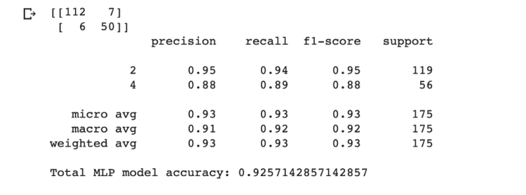
- For extra visualization I present a confusion matrix that compares my predictions with the correct labels. (If you are not familiar with confusion matrices, for now just know that values along the diagonal represent correct predictions). This also leads us to an accuracy percentage by dividing the sum of correct predictions by the sum of values in the y_test vector.
Step 4: Visualize Linear Separability by Plotting a Learning Curve
What is Linear Separability?
Linear Separability refers to checking if one can completely separate classification of data in an n-dimensional space using N — 1 dimensions. For example, if classification of data is plotted on a single line, if the classes can be separated by a single point it is linearly separable. Another example is if you can separate classification data by a straight line on a 2-D plot.
Our Learning Curve
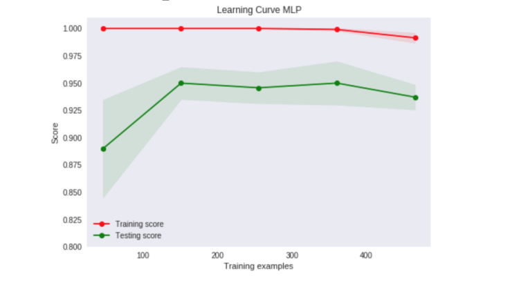
From looking at this specific learning curve, the perceptron does not converge and so we can determine that the data in this case is not linearly separable, and with that knowledge, we know that we should use at least one hidden layer in our model.
Step 5: Building a Support Vector Machine on same dataset
We start building our support vector machine by establishing a svm under the variable vectorMachine with a linear kernel function. We will use a linear function as our SVM will predict on a 2-dimensional space, as our input vector contains one dimensional data.
Trending AI Articles:
1. Part-of-Speech tagging tutorial with the Keras Deep Learning library
2. Tutorial: Stereo 3D reconstruction with openCV using an iPhone camera
What is a kernel function?
This is a key attribute of the SVM model as it is a mathematical function that transforms data into higher dimensional space so that the machine can perform faster calculations (i.e. like creating vectors that serve as boundaries for specific classifications in data).

How does a support vector machine work?
After the kernel function has been applied to our data and we have an appropriate n-dimensional space, the support vector machine finds an optimal hyperplane, or separating line, between the classifications, but as close to the nearest classification as possible. After the machine has determined the hyperplane it classifies the data, by quickly configuring if incoming data is on either side of the hyperplane.
Next, we fit (train) the machine with a function that operates on our testing sets. After the SVM is fitted and ready for new data, we use the predict() function provided by Sci-Kit Learn and create a vector of predictions on the prime testing set of the Wisconsin Breast Cancer data. And just like the Multilayer Perceptron model above, we can determine model accuracy by dividing the sum of correct predictions the SVM makes by the length of the label vector, y_test.

Although, it’s close, the SVM model generally is getting better results!
Why does a SVM model work better on this data than a Multilayer perceptron?
By default, SVM’s usually have higher prediction accuracy than a multilayer perceptron. SVM’s might have higher runtime as there are calculations it performs that are advanced like translating n-dimensional space using kernel functions. But it usually does a very good job in its predictions.
In this dataset, we are classifying breast cancer outcomes by various attributes that are observed with each patient. The two classifications our models are predicting are either benign or malignant. This data specifically is prime for an SVM model, as it can easily find the perfect hyperplane after translating the data using its kernel function.
Step 6: Evaluating the SVM Model with 5-fold Cross Validation Techniques
The purpose of this is to cross validate the accuracies the SVM model has on K different versions of the dataset. In this case 5 different versions.
How I think of cross-validation techniques
I like to envision 5-fold cross validations as almost like a balance beam visual, where one side is the training portion and the other side is the testing portion of the data, and we have 5 equal weights dispersed across the balance beam. We start with 1 on testing side and 4 on the training side and then we take from training to testing with K iterations training our model. So eventually every combination will be tried and it is quite thorough in determining model accuracy.
Following the code:
- We split our data into 5-fold groups
- We pre-process the data, just like we did when we initialized our vectors for the two models above
- Then we train the model we are testing based on these newly split training sets
- Predict accuracy exactly like above, but this time it is with the K-split, in our case 5-split, training sets.

Conclusion
I found this experiment very conclusive! It performed pretty much how it was supposed to:
- The Multilayer Perceptron performed pretty well on the data — upwards of 90%.
- The superior performing SVM stole the show, but barely, with a little more predictive accuracy
- When put to a thorough test, the SVM showed its strength in the cross-validation evaluation with a 99% percent accuracy.
As always, thanks for reading! I learned a lot more about the differences between the two models as I was documenting this project so I hope you learned a bit too.
Don’t forget to give us your ? !


Comparing SVM and MLP Machine Learning Models was originally published in Becoming Human: Artificial Intelligence Magazine on Medium, where people are continuing the conversation by highlighting and responding to this story.
