
In this article, I will try to predict the locations of deforestation in Amazon Forests using Ridge, Decision Tree, Random Forest and XGBoost regression models.
Introduction
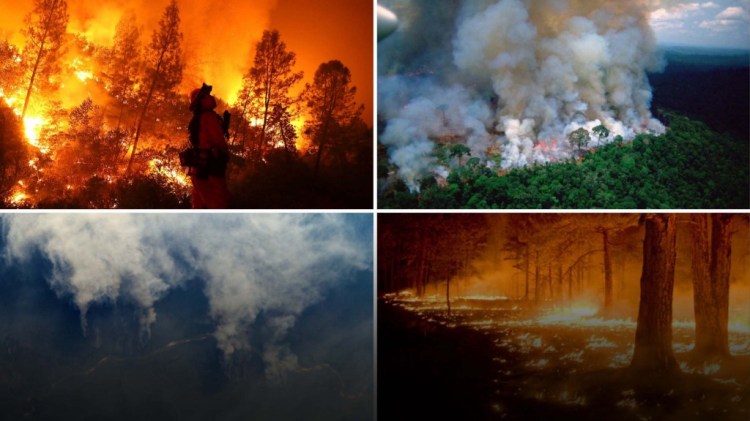
Deforestation is a clearing, destroying, or removing trees due to farming, mostly cattle, logging, for materials and development, mining, and drilling. All of this combined responsible for more than half of all deforestation. Over the past 50 years, nearly 17 percent of the Amazon rain forest has been lost and losses have recently been on the rise.
Exploring the domain
While exploring and analyzing the data I noticed a tendency that most of the deforestation happen not far from places where it occurred in the past. Mostly it is connected with farms, where more space needed for the cattle to grow, logging to produce more paper or wood materials and other work.
Check my web app for more visual analysis & a little demonstration.

Dataset
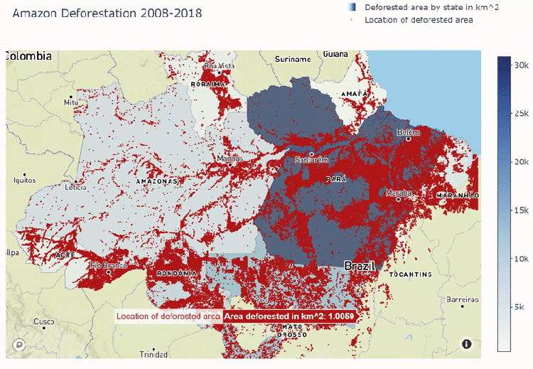
I took the dataset from terrabrasilis.dpi.inpe.br/en where records quantified deforested areas larger than 6.25 hectares from 2008 to 2018 discretized per year.
The dataset includes columns: gid — unique identifier of each feature;
origin_id — unique identifier for traceability of the feature in the origin for geo data;
geo data — feature composed of one or more polygons — geometry obtained by visual interpretation of satellite image;
uf — state abbreviation;
pathrow — scene code formed by line of the satellite (the land is is divided in squares as in 2d space);
mainclass— name of the main class assigned to the feature;
class_name — name of the specific class assigned to the feature;
dsfnv — indicates if there was a cloud in the previous year about the feature;
julday— julian day;
view_date — date of the scene used to obtain the feature;
year — year of deforestation, used to facilitate queries to the areakm database;
areakm— area calculated for the feature in km²;
scene_id — identifier of the scene in the database, used for publish_year queries;
publish_year — used to allow the publication of data on the GeoServer with temporal dimension.
Wrangling and Cleaning the Data
I used pandas profiling to look at my data and features closely and see the distribution, check for cardinality, zeros and nulls. Most of the features didn’t make sense to me in predicting the locations of the deforested area except for the states and view_date, also I took into consideration area in kilometres squared (areakm_squared), some states have more deforested areas than others. Geo data had the longitude and latitude, the centroid of the deforested area, which I decided to be the targets for my predictions.

Visualizing the data
Mapbox plot below shows deforestation areas spread out through all Amazon states. We see that most of the deforestation comes to Para state and least goes to Amapa.
The Process
The aim is to predict the location of an area (centroid)where deforestation most likely to occur. I decided to try different models for my predictions and see which performs better. Since it is a spatial data, for the sake of simplicity I decided to treat the location as it is in 2D space and not the sphere and predict latitude and longitude as two separate values using two different models.
Top 4 Most Popular Ai Articles:
3. Real vs Fake Tweet Detection using a BERT Transformer Model in few lines of code
I made a time-based split of the data – train, validation and test. Train data 2008–2015, validation 2016, and test 2017–2018. After cleaning up and feature engineering, I ended up with only five features: [‘areakm_squared’, ‘day’, ‘month’, ‘year’, ‘states’].
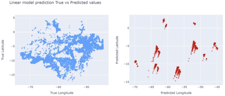
Ridge Model
The first model I tried is Ridge model, which of course is not so good at predicting coordinates, but at least I wanted to see where I stood. For the encoding I chose TargetEncoder, also I scaled values with StandardScaler, and used SelectKBest for the features.
For metrics on validation set, I chose MAE (mean absolute error), RMSE (root mean absolute error)and R² score (r-squared).
Ridge model validation MAE: 1.3207 lat
Ridge model validation MAE: 1.8468 lon
Ridge model Validation RMSE: 2.8329 lat
Ridge model Validation RMSE: 5.4658 lon
Ridge model Validation R^2 coefficient: 0.7949 lat
Ridge model Validation R^2 coefficient: 0.8801 lon
The plot below shows the predictions on validation set, and as I expected, it performed poorly, even though the metrics look good.
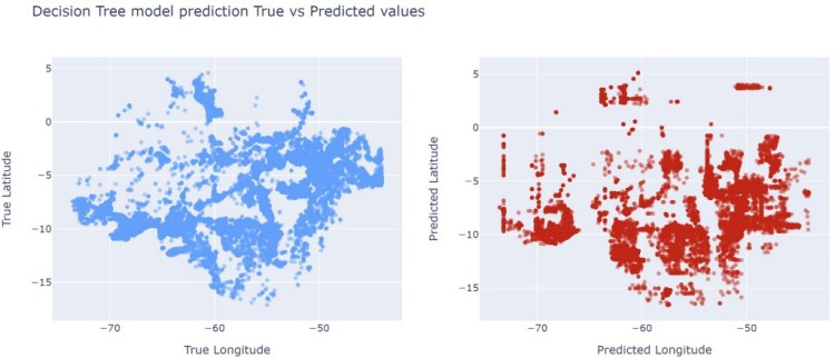
Decision Tree Model
The next model I tried is DecisionTreeRegressor model. I used TargetEncoder and default hyperparameters. For validation data I used the same metrics:
Decision Tree validation MAE: 2.1791 lat
Decision Tree validation MAE: 3.3861 lon
Decision Tree Validation RMSE: 7.4978 lat
Decision Tree Validation RMSE: 19.2732 lon
Decision Tree Validation R^2 coefficient: 0.4571 lat
Decision Tree Validation R^2 coefficient: 0.5773 lon
DecisionTreeRegressor performed a little better than Ridge model, we can see predictions are closer to true coordinates, however, it is still far from true values.
Random Forest Model
For the RandomForestRegressor model, I used hyperparameter tuning. I applied RandomizedSearchCV to choose the best hyperparameters. The best hyperparameters for latitude are:
{'randomforestregressor__max_features': 0.31276908252447455,
 'randomforestregressor__n_estimators': 108,
 'simpleimputer__strategy': 'mean',
 'targetencoder__min_samples_leaf': 54}
and for longitude:
{'randomforestregressor__max_features': 0.6404643986998269,
 'randomforestregressor__n_estimators': 186,
 'simpleimputer__strategy': 'median',
 'targetencoder__min_samples_leaf': 329}
With the RandomForestRegressor model and hyperparameter tuning I got much better scores:
Random Forest Validation MAE: 1.6633 lat
Random Forest Validation MAE: 2.9025 lon
Random Forest Validation RMSE: 4.3909 lat
Random Forest Validation RMSE: 11.7841 lon
Random Forest Validation R^2 coefficient: 0.6821 lat
Random Forest Validation R^2 coefficient: 0.7415 lon
And the graph looks better:

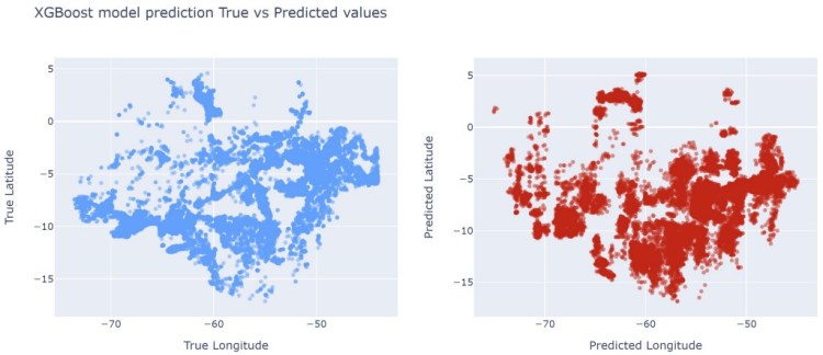
RandomForestRegressor made the best predictions so far. The last model I tried is XGBoostRegressor model. I picked OrdinalEncoder this time to transform the data and applied early_stopping to see what are the best n-estimators to use.
The MAE in XGBoostRegressor is higher and R²-score is lower than in the Random Forest model:
XGBoost Validation MAE: 1.9527 lat
XGBoost Validation MAE: 3.1559 lon
XGBoost Validation RMSE: 6.0368 lat
XGBoost Validation RMSE: 14.1507 lon
XGBoost Validation R^2 coefficient: 0.5625 lat
XGBoost Validation R^2 coefficient: 0.6885 lon
Let’s see how XGBoostRegressor model looks like on the graph:
The best model out of all I tried was RandomForestRegressor, I got less MAE, RMSE loss was less, and R²-score was higher, so I decided to use this model for predictions on my test set.
Feature Selection and Model Interpretation

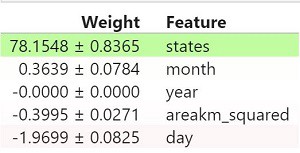
Before applying my model on the test set, I wanted to see an overall contribution of features in RandomForestRegressor model. I ran Permutation Importance from library eli5.sklearn. It showed only one feature that contributed the most in predicting coordinates which is ‘states’, and some of the features contributed even negatively, like ‘areakm_squared’ and ‘day’ in case of longitude values.
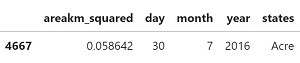
Permutation Importance only gives general information about feature contribution. Let’s break down how the model works for an individual prediction. I used SHAP Values to break down a prediction to show the impact of each feature and it’s positive or negative impact. As an example, let’s take a random row from our validation set:
# take a random row from val set
row = X_val.iloc[[200]]
row
We got nice interpretation for latitude and longitude and how much each feature contributed:
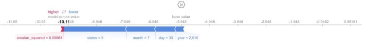
In predicting latitude value ‘states’, ‘month’, ‘day’, and ‘year’ features contributed in a negative direction from the mean, while ‘areakm_squared’ and contributed in a positive direction towards the mean.
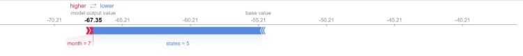
In the case with longitude, we can see that ‘states’, ‘areakm_squared’ and ‘day’ features contributed negatively, however ‘month’ and ‘year’ contributed in positively.
Applying the best model to test set
Final predictions with RandomForestRegressor model on my test set didn’t perform that good for latitude values, however, did better for longitude comparing to validation set scores. There is a big difference in R² score.
Random Forest MAE: 1.9317 lat
Random Forest MAE: 2.6541 lon
Random Forest RMSE loss: 5.9613 lat
Random Forest RMSE loss: 11.3523 lon
Random Forest R^2 coefficient: 0.5621 lat
Random Forest R^2 coefficient: 0.7733 lon
Let’s look at the final predictions on the scatter plot and compare to true ones. In some places it did okay, but mostly it didn’t do very well.

Conclusion
In my opinion, to predict coordinates of locations is not so easy, because they are two values representing 3D space. Even that I treated coordinates as in 2D plane and used several models to see which ones perform better I didn’t have very good results. Also, my dataset didn’t have many features to use for predictions and I ended up with only five. It would be nice if dataset would have some features like population density, distance from a big city to a place of deforestation, causes of deforestation, and maybe some others could help to identify future locations of deforestation.
Note:
This project was done for Lambda School as an optional part of the Data Science curriculum.
For my visualizations, I used Plotly Scatter Mapbox.
Dataset is here: http://terrabrasilis.dpi.inpe.br/en/download-2/
Don’t forget to give us your ? !


Can We Predict Deforestation in Amazon Forests with Machine Learning? was originally published in Becoming Human: Artificial Intelligence Magazine on Medium, where people are continuing the conversation by highlighting and responding to this story.
