Microsoft Azure Machine Learning x UdacityLesson 3 Notes

Microsoft Azure Machine Learning x Udacity — Lesson 3 Notes

Detailed Notes for Machine Learning Foundation Course by Microsoft Azure & Udacity, 2020 on Lesson 3 — Model Training

This lesson is about how to prepare data and transform it into trained machine learning models. This lesson will also introduce you to ensemble learning and automated machine learning.

Data Import & Transformation

Data Wrangling:

Cleaning, restructuring, enriching data to transform it into a suitable format for training machine learning models. This is an iterative process.

Steps:

• Discovery & Exploration of data
• Transformation of raw data
• Publish data

Managing Data:

Datastores:

A layer of abstraction. It stores all the information needed to connect to a particular storage device

Datasets:

Resources for exploring, transforming, managing data. A reference to a point in storage.

Data Access Workflow:

• Create a datastore
• Create a dataset
• Create a dataset monitor (critical to detecting issues in data, e.g. Data Drift)

Introducing Features

• Feature Selection
• Dimensionality Reduction

Feature Engineering

• Core techniques
• Various places to apply feature engineering: 1) datastores 2) a python library 3) during model training
• Used more often in classical machine learning

Feature Engineering Tasks:

• Aggregation: sum, mean, count, median, etc (math formulas)
• Part-of: extract a part of a certain data structure, e.g. a part of date like hour
• Binning: group entities into bins and apply aggregations on them
• Flagging: deriving Boolean conditions
• Frequency-based: calculate the various frequencies of occurrence of data
• Embedding or Feature Learning: a relatively low-dimensional space into which you can translate high-dimensional vectors
• Deriving by Example: aim to learn values of new features using examples of existing features

Feature Selection

Given an initial dataset, create a number of new features. Find out useful and filter out features.

Reasons for Feature Selection:

1. Eliminate redundant, irrelevant, or highly correlated feature

2. Dimensionality reduction

Dimensionality Reduction Algorithms:

• Principle Component Analysis (PCA): Linear technique with more of a statistical approach.
• t-Distributed Stochastic Neighboring Entities (t-SNE): A probabilities approach to reduce dimensionality. The target number of dimensions with t-SNE is usually 2–3 dimensions. It is used a lot for visualizing data.
• Feature Embedding: Train a separate machine learning model to encode a large number of features into a smaller number of features also super-features.

All the above are also considered to be Feature Learning techniques.

Azure Machine Learning Prebuilt Modules Available:

• Filter-Based Feature Selection: Helps identify the columns in input dataset that have a dataset that has the greatest predictive power
• Permutation Feature Importance: Helps determine the best features to use in a model by computing a set of feature-important-scores for your dataset

Data Drift

Data Drift is a change in the input data for a model. Over time, data drift causes degradation in the model’s performance, as the input data drifts farther and farther from the data on which the model was trained.

Trending AI Articles:

1. Machine Learning Concepts Every Data Scientist Should Know

2. AI for CFD: byteLAKE’s approach (part3)

3. AI Fail: To Popularize and Scale Chatbots, We Need Better Data

4. Top 5 Jupyter Widgets to boost your productivity!

It is the top reason why accuracy drops over time. Detecting data drift helps identify model performance issues and also enables us to trigger retraining processing to avoid that.

Causes of Data Drift:

1. Upstream process changes e.g. A sensor is replaced, causing the units of measurement to change (e.g., from minutes to seconds)
2. Data quality issues e.g. sensor breaks
3. Natural data drift: data is not static e.g. customer behavior
4. Covariate shift: changes in the relationship between features

Dataset Monitors:

Dataset Monitors can be set up to provide alerts to assist in detecting data drifts over a dataset. They will help not only create models that are good at a given point in time but also models that keep their level of performance in time.

Monitoring for Data Drift:

Monitoring/detecting early enough cases of data drift are critical to maintaining a healthy state of the model. Data drift algorithm provides an overall measure of the change that occurs within data.

The process of monitoring for data drift involves:

• Specifying a baseline dataset — usually the training dataset. used originally for training
• Specifying a target dataset — usually the input data for the model
• Comparing these two datasets over time, to monitor for differences

Scenarios for setting up data drift monitors in Azure ML:

1. Monitoring a models input data for drift from the model’s training
2. Monitoring a time-series dataset for drift from a previous time period.
3. Performing analysis of past data. Typically done on historical data to better understand the dynamics of the data, better decision-making to improve model

Understanding Data Drift Results:

Results are produced in charts — Drift Overview shows the following set of charts:

1. Data Drift Magnitude: percentage between the baseline and target dataset over time and ranges between 0–100% (where 0 indicates identical datasets and 100 indicates completely separable datasets).

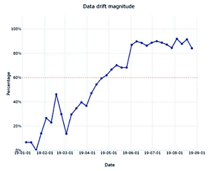
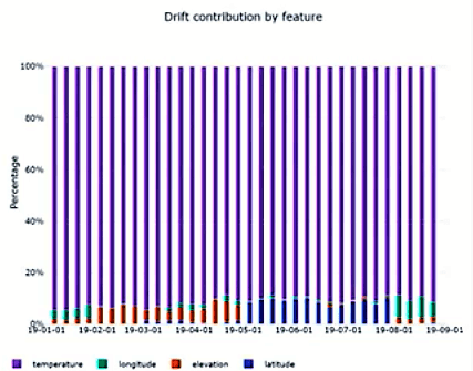
1. Drift Contribution by Feature: helps understand which particular features of your dataset have contributed most to the data drift process. Identifying which those features are is very important because then they can be better understood, i.e.1) the way they evolve through time, and 2) how to use them in the most appropriate way in model training.

Here are a couple of different types of comparisons you might want to make when monitoring for data drift:

• Comparing input data vs. training data. This is a proxy for model accuracy; that is, an increased difference between the input vs. training data is likely to result in a decrease in model accuracy.
• Comparing different samples of time series data. In this case, you are checking for a difference between one time period and another. For example, a model trained on data collected during one season may perform differently when given data from another time of year. Detecting this seasonal drift in the data will alert you to potential issues with your model’s accuracy.

Model Training Basics

The goal of the Model Training process is to produce a trained model that you can later use to predict. We want to be able to give the model a set of input features, X, and have it predict the value of some output feature, y.

It is important to establish the problem to be solved e.g a classification or regression problem. The framing of the problem will influence both the choice of algorithms in the training process as well as the various approaches to take to get to the desired result.

The important prerequisite is to understand, transform data, create new features, selecting features that are most relevant to the training process. Once we have both problem time and training features defined, next steps are:

1. Decide whether to scale or encode your data
2. Splitting data (i.e. Training, Validation, and Test dataset)

Parameters and Hyperparameters:

When we train a model, a large part of the process involves learning the values of the parameters of the model. For example, earlier we looked at the general form for linear regression:

y = B0 + B1*x1 + B2*x2 + B3*x3 … + Bn*xn

The coefficients in this equation, B_0 … B_nB0​…Bn​, determine the intercept and slope of the regression line. When training a linear regression model, we use the training data to figure out what the value of these parameters should be. Thus, we can say that a major goal of model training is to learn the values of the model parameters.

In contrast, some model parameters are not learned from the data. These are called hyperparameters and their values are set before training. Here are some examples of hyperparameters:

• The number of layers in a deep neural network
• The number of clusters (such as in a k-means clustering algorithm)
• The learning rate of the model

We must choose some values for these hyperparameters, but we do not necessarily know what the best values will be prior to training. Because of this, a common approach is to make the best guess, train the model, and then tune adjust or tune the hyperparameters based on the model’s performance.

Splitting the Data:

As mentioned in the video, we typically want to split our data into three parts:

• Training data
• Validation data
• Test data

We use the training data to learn the values for the parameters. Then, we check the model’s performance on the validation data and tune the hyperparameters until the model performs well with the validation data. We can adjust this hyperparameter and then test the model on the validation data once again to see if its performance has improved.

Finally, once we believe we have our finished model (with both parameters and hyperparameters optimized), we will want to do a final check of its performance — and we need to do this on some fresh test data that we did not use during the training process.

Model Training in Azure Machine Learning

Azure Machine Learning Service provides a comprehensive environment to implement model training processes, giving you a centralized place to work with all the artifacts involved in the process. It is also called a Machine Learning Managed Service and provides a platform which 1) simplifies the implementation of various tasks and 2) offers all the necessary kinds of services that will help create the best possible machine learning models. It provides out of the box managed services that help implement every step of the data science process.

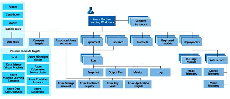
Taxonomy of Azure Machine Learning:

Several types of artifacts and several classes of concepts related to the implementation of the various steps of data science.

Workspace: The centralized place for working with all the components of the machine learning process. Everything in Azure Machine Learning revolves around this concept and is the very first thing to be created in the pipeline.

Compute Instances: A cloud-based workstation that gives you access to various development environments, such as Jupyter Notebooks.

Datasets: A key component in the data preparation and transformation processes that makes data available to Machine Learning processes.

Experiment: A container that helps you organize the model training process and group various artifacts/tasks related to Machine Learning processes run within Azure.

Run: A process that is executed in one of the compute resources e.g. model training, model validation, feature engineering. Every Run will output a set of artifacts: snapshots of data, output files, metrics, and logs.

Compute Targets: Machine Learning processes on a large variety of environments:

1. Local environments
2. Remote environments: Native Azure, Azure Data Dake AnalyticS

Registered Models: A service that provides snapshots and versioning for your trained models. After a model is created, it gets registered into the Model Registry. Note: Versioning is also important for Models, just like datasets, so that end-to-end traceability is achievable.

Deployment: Either in the form of web services or other types of environments, IoT Edge, etc.

Model Telemetry: Collect telemetry from live running models (model predictions using production input data).

Service Telemetry: Collect telemetry from live running services (model input data from web services)

Training Classifiers

In a classification problem, the outputs are categorical or discrete.

There are three main types of classification problems:

1. Binary Classification: True/False, 0 or 1. e.g Anomaly detection, Fraud Detection
2. Multi-Class Single-Label Classification: output is categorized between 3 or more. e.g. recognition of written numbers.
3. Multi-Class Multi-Label Classification: multiple categories and output can belong to more than one. e.g. text tagging

Examples of Classification Algorithms:

1. Logistic Regression
2. Support Vector Machine (SVM)

Training Regressors

In a regression problem, the output is numerical or continuous.

There are two main types of regression problems:

1. Regression to arbitrary values: prediction based on various inputs. No boundary defined for the output
2. Regression to vales between 0 and 1: bound the outputs between the interval of 0 and 1 and assigns it as a probability

Examples of Regression Algorithms:

1. Linear Regressor
2. Decision Forest Regressor

Evaluating Model Performance

The evaluation of a Machine Learning model is a critical step through which you calculate a set of performance metrics in order to assess its performance — such as the predictive power and accuracy of the model.

we need to split off a portion of our labeled data and reserve it for evaluating our model’s final performance. We refer to this as the test dataset.

The test dataset is a portion of labeled data that is split off and reserved for model evaluation.

When splitting the available data, it is important to preserve the statistical properties of that data. the data in the training, validation, and test datasets need to have similar statistical properties as the original data to prevent bias in the trained model. Splitting the data up randomly will help ensure that the two datasets are statistically similar.

Confusion Matrices

A confusion matrix gets its name from the fact that it is easy to see whether the model is getting confused and misclassifying the data.

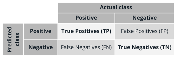
• True positives are the positive cases that are correctly predicted as positive by the model
• False positives are the negative cases that are incorrectly predicted as positive by the model
• True negatives are the negative cases that are correctly predicted as negative by the model
• False negatives are the positive cases that are incorrectly predicted as negative by the model

Evaluation Metrics for Classification

Accuracy: measures the goodness of a classification model as the proportion of true results to total cases

(TP+TN) ​/ (TP+FP+FN+TN)

Precision: the proportion of true results overall positive results

TP / TP+FP​

Recall: the fraction of all correct results returned by the model

TP / TP+FN​

F1-Score: computed as the weighted average of precision and recall between 0 and 1, where the ideal F1-Score value is 1

2∗Precision+Recall / Precision∗Recall​

Note: None of these independently are enough to provide an accurate measurement of metrics for classification and are used in pairs to get a complete image of a classification algorithm.

Model Evaluation Charts

When evaluating models, a level of understanding can be quickly gained using charts:

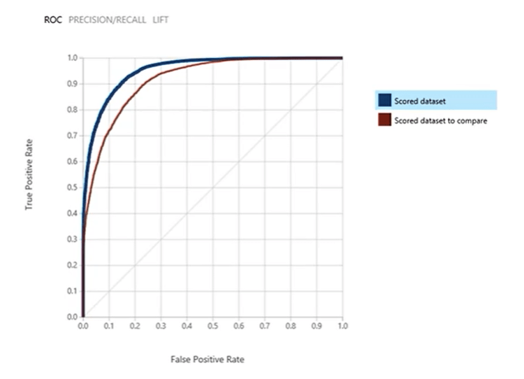
1. Receiver Operating Characteristics (ROC) Chart: a graph of the rate True Positives against the rate of False Positives. A metric that is derived from this is the Area Under the Curve (AUC).

• AUC measures the area under the ROC curve plotted with true positives on the y-axis and false positives on the x-axis. This metric is useful because it provides a single number that lets you compare models of different types. An AUC of 0.5 indicates random guessing, while an AUC of 1.0 indicates perfect classification hence, the area under the curve should always fall between the range of 0.5 and 1.0.

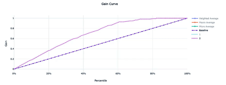
1. Gain and Lift Charts: deals with ordering with rank, ordering the prediction probabilities, and measure how much better the classifier can perform. The diagonal line corresponds to random guessing; the other line corresponds to performance when a trained classifier is used. Ideally, the latter line should be as far away from the former as possible.

Evaluation Metrics for Regression

1. Root Mean Squared Error (RMSE): the square root of the squared differences between the predicted and actual values. It creates a single value that summarizes the error in the model. By squaring the difference, the metric disregards the difference between over-prediction and under-prediction.
2. Mean Absolute Error (MAE): Average of the absolute difference between each prediction and the true value. It measures how close the predictions are to the actual outcomes; thus, a lower score is better.
3. R-Squared: known as the coefficient of determination. How close the regression line is to the true values.
4. Spearman Correlation: Strength and direction of the relationship between predicted and actual values.

Model Evaluation Charts

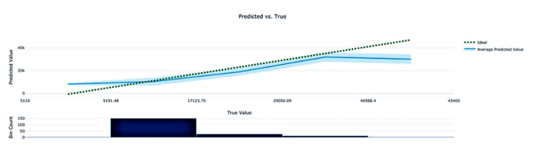
1. Predicted vs. True Chart: displays the info/relationship between the predicted and the true value. Shown below, the perfect regressor is represented by the diagonal line whereas the predicted line is the one below it indicating errors. At the bottom of the chart, the histogram shows how the true values are distributed in your prediction results.

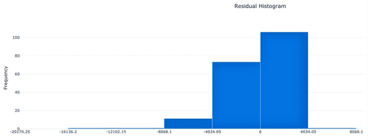
1. Histogram of Residuals: represents the distribution of the true value subtracted by the predicted value hence, the difference. When the model has a fairly low bias, the histogram should approach more or less a normal distribution (bell-shaped) which one should try to achieve.

Strength in Numbers

No matter how well-trained an individual model is, there is still a significant chance that it could perform poorly or produce incorrect results. To train multiple instances of machine learning models and capture their collective wisdom in a way that would alleviate the potential issues produced by single models. there are two main approaches along these lines. Both use the principle of Strength in Numbers to reduce the potential error/bias of individual machine learning models. We use the strength of a large number of trained models with the purpose to improve the accuracy of predictions.

Ensemble Learning

It combines multiple machine learning models to produce one predictive model. There are three main types of ensemble algorithms:

1. Bagging or Bootstrap Aggregation

• Helps reduce overfitting for models that tend to have high variance (such as decision trees)
• Uses random subsampling of the training data to produce a bag of trained models.
• The resulting trained models are homogeneous
• The final prediction is an average prediction from individual models

2. Boosting

• Helps reduce bias for models.
• In contrast to bagging, boosting uses the same input data to train multiple models using different hyperparameters.
• Boosting trains model in sequence by training weak learners one by one, with each new learner correcting errors from previous learners hence, constantly improving the model.
• The final predictions are a weighted average from the individual models.

3. Stacking

• Trains a large number of completely different (heterogeneous) models
• Combines the outputs of the individual models into a meta-model that yields more accurate predictions

Strength in Variety: Automated ML

Automated Machine Learning plays on the principle of Strength in Variety and, as the name suggests, automates many of the iterative, time-consuming, tasks involved in model development (such as selecting the best features, scaling features optimally, choosing the best algorithms, and tuning hyperparameters). Automated ML allows data scientists, analysts, and developers to build models with greater scale, efficiency, and productivity — all while sustaining model quality. Automated ML explores combinations that help find the best performing combination to improve the accuracy of a prediction. Automated ML is not a replacement for a data scientist but a way to get a baseline model and then try other approaches to get superior performance.

Summary

In this lesson, you’ve learned to perform the essential data preparation and management tasks involved in machine learning:

• Data importing and transformation
• The use of datastores and datasets
• Versioning
• Feature engineering
• Monitoring for data drift

The second major area we covered in this lesson was model training, including:

• The core model training process
• Two of the fundamental machine learning models: Classifier and regressor
• The model evaluation process and relevant metrics

The final part of the lesson focused on how to get better results by using multiple trained models instead of a single one. In this context, you learned about ensemble learning and automated machine learning. You’ve learned how the two differ, yet apply the same general principle of “strength in numbers”. In the process, you trained an ensemble model (a decision forest) and a straightforward classifier using automated Machine Learning.

Don’t forget to give us your ? !

---

Microsoft Azure Machine Learning x Udacity — Lesson 3 Notes was originally published in Becoming Human: Artificial Intelligence Magazine on Medium, where people are continuing the conversation by highlighting and responding to this story.

Via https://becominghuman.ai/microsoft-azure-machine-learning-x-udacity-lesson-3-notes-8498661210c4?source=rss—-5e5bef33608a—4