

Hello world! Hope you’re doing great today. In this article I would like to do a project related to Natural Language Processing (NLP). The project itself is not going to be very complicated as what we are gonna do is just a simple binary classification task.
So we know that Coronavirus is still around up until the time when I write this article. And thus, it’s obviously possible that there are also plenty of fake news related to that topic coming into the society. So the objective of this project is to create a machine learning model which is able to detect whether a news is fake or real.
Note: full code available in the end of this article.
Let’s start with some imports. I will explain them later on.
import re
import pandas as pd
import numpy as np
import matplotlib.pyplot as plt
import seaborn as sns
from sklearn.feature_extraction.text import CountVectorizer
from sklearn.naive_bayes import MultinomialNB
from sklearn.model_selection import train_test_split
from sklearn.metrics import confusion_matrix
from nltk.tokenize import word_tokenize
from nltk.corpus import stopwords
Data collection & analysis
Before I go any further, I wanna inform you that the project that I’m going to explain here is inspired by the this article. The author of that article uses logistic regression to do the classification and obtain 93% of accuracy towards test data. On the other hand, here in my project I would like to employ Naïve Bayes classifier instead and see if I can obtain higher accuracy using this approach with the exact same dataset. You can download the COVID-19 news dataset from here.
Now after downloading the dataset, let’s do a simple Exploratory Data Analysis (EDA) to find out important (and probably interesting) things in the dataset.
df = pd.read_csv('covid_fake_news.csv')
print(df.shape)
df.head()

After running the code above, we should get an output like the following image and the shape of the data frame df, which is (1164, 4). It says that our dataset consists of 1164 rows in which each of those has 4 attributes.
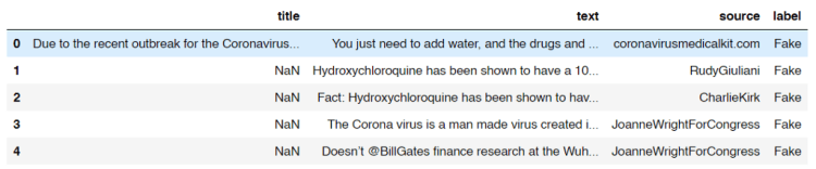
Look at the title column. Here we see that some of the titles are missing. Now I got a feeling that probably there are also some other missing stuff in the dataset which might affect the overall performance of our model. So I decided to count the number of those missing values from each column.
print("No of missing title\t:", df[df['title'].isna()].shape[0])
print("No of missing text\t:", df[df['text'].isna()].shape[0])
print("No of missing source\t:", df[df['source'].isna()].shape[0])
print("No of missing label\t:", df[df['label'].isna()].shape[0])
And here is the result:
No of missing title     : 82
No of missing text      : 10
No of missing source    : 20
No of missing label     : 5
Now we know that actually some of the cells in our data frame contains NaN (Not a Number) values. By knowing this fact, what I wanna do now is assigning an empty string (‘’) to all those cells like this:
df = df.fillna(‘’)
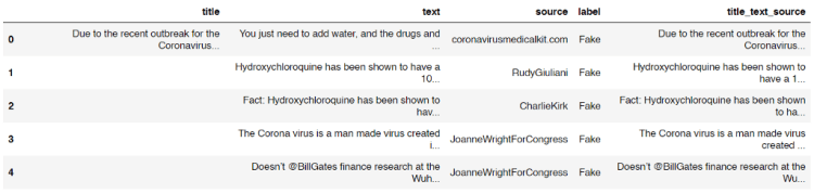
Next, the title, text and source columns are then going to be concatenated which the result is stored in another new column called title_text_source . This new column in our data frame df is going to be our raw X data.
df[‘title_text_source’] = df[‘title’] + ‘ ‘ + df[‘text’] + ‘ ‘ + df[‘source’]
df.head()
Now our data frame is going to look something like this:
On the other hand, all samples with missing values in label column will just be dropped since I got no idea whether each of those is real or fake news. The following code is my approach to delete them.
df = df[df[‘label’]!=’’]
print(df['label'].unique())
Now the output after running the code above shows that all our non-labeled data are already removed as there is no empty string appears as the unique value in label column.
array(['Fake', 'TRUE', 'fake'], dtype=object)
But wait! We got another problem here! You can see the output above that our labels are not uniform. So then it’s really necessary to fix this. Here I decided to put those into 2 classes, namely TRUE and FAKE. Below is the code to do so:
df.loc[df['label'] == 'fake', 'label'] = 'FAKE'
df.loc[df['label'] == 'Fake', 'label'] = 'FAKE'
Now that all fake and Fake labels are already converted into FAKE. You can check it by running df[‘label’].unique() again. Since up to this step we already got 2 unique labels (only FAKE and TRUE), we can calculate the number of data of each class using the following code:
no_of_fakes = df.loc[df['label'] == 'FAKE'].count()[0]
no_of_trues = df.loc[df['label'] == 'TRUE'].count()[0]
print(no_of_fakes)
print(no_of_trues)
After running the code above we should get an output like this:
No of fake data:  575
No of true data:  584
Now we can see here that the numbers of fake and true data are almost equal. And this is a good news because any machine learning algorithm will work best if the number of data of all classes are balanced.
Trending Bot Articles:
2. Chatbots 2.0: Simplifying Customer Service with RPA and AI
Text preprocessing
Lemme print out our latest data frame df again using df.head() command.
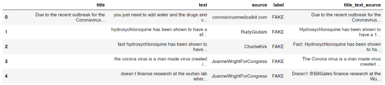
We know that there are probably plenty of useless words or characters which exist in the title_text_source column, such as Twitter user name and stop words (i.e. and, or, if, the, into, etc). Here in this step we are going to get rid of those words using the clean() function I defined below.
stop_words = set(stopwords.words('english'))
def clean(text):
    # Lowering letters
    text = text.lower()

    # Removing html tags
    text = re.sub(r'<[^>]*>', '', text)

    # Removing twitter usernames
    text = re.sub(r'@[A-Za-z0-9]+','',text)

    # Removing urls
    text = re.sub('https?://[A-Za-z0-9]','',text)

    # Removing numbers
    text = re.sub('[^a-zA-Z]',' ',text)

    word_tokens = word_tokenize(text)

    filtered_sentence = []
    for word_token in word_tokens:
        if word_token not in stop_words:
            filtered_sentence.append(word_token)

    # Joining words
    text = (' '.join(filtered_sentence))
    return text
So the first thing I do in the code above is to create a set of all stop words in English stored in stop_words variable. Next, I define a clean() function which takes a text as the only parameter. After that, this text is going to be processed, mostly using re (Regular Expression) module. You can see the comments in the code for the details. I also perform tokenization to the text in order to filter out stop words before returning the cleaned text as the output.
Before actually applying the function to each rows in the title_text_source column, I want to check whether the function works as expected like this:
print(clean('Hello World 22 Ardi, and or if they 3878, I am @Ardi'))
And yes, it the function works properly as it does remove all unnecessary words.
'hello world ardi'
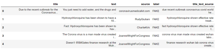
Now, to clean all texts stored in title_text_source column, we can simply use apply() method to that column like this:
df['title_text_source'] = df['title_text_source'].apply(clean)
After running the code above you will see that all texts in the column are already cleaned.
Count vectorizer
We know that any machine learning or deep learning algorithms can not directly work with words. Thus, it’s obviously necessary to convert all texts in title_text_source into numbers. In this project, I am going to use count vectorizer as the approach to do it. The concept of count vectorizer itself is pretty trivial, since we only need to count the occurrence of each word for every single text in order to create a feature vector of that. If you still don’t get the idea of count vectorizer I recommend you to read this simple explanation.
The implementation is very simple thanks to the existence of Scikit-learn module.
vectorizer = CountVectorizer()
X = vectorizer.fit_transform(df['title_text_source'].values)
X = X.toarray()
Look at the code above. The first thing we do is to initialize a count vectorizer object which I call it as vectorizer. Then in the next two lines I use this vectorizer to convert all values of title_text_source column (which is still in form of text) into array of word occurrences. Now if we try to print out this X variable, we will get the following output:
array([[0, 0, 0, ..., 0, , 0],
       [0, 0, 0, ..., 0, 0, 0],
       [0, 0, 0, ..., 0, 0, 0],
       ...,
       [0, 0, 0, ..., 0, 0, 0],
       [0, 0, 0, ..., 0, 0, 0],
       [0, 0, 0, ..., 0, 0, 0]], dtype=int64)
The shape of the array above is (1159, 21117) which represents the number of samples and the feature vector size of each sample respectively.
Naïve Bayes classifier
Up to this point we already got feature vectors for all samples stored in X variable. To make things more intuitive, I will also define y variable, which I will use it to store all ground truths (a.k.a. labels).
y = df['label'].values
Now we can use y as the replacement of df[‘label’].values
Before training a classifier, we are going to split the data into train and test, where 20% of the entire samples in the dataset are going to be used to test the overall performance of the model. This splitting can easily be done using train_test_split function taken from Sklearn module:
X_train, X_test, y_train, y_test = train_test_split(X, y, shuffle=True, test_size=0.2, random_state=11)
After running the code above, we got 4 new variables which I guess all of those are self-explanatory.
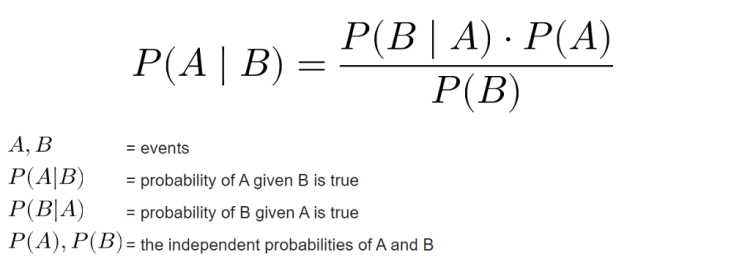
Now as the data already split it’s time to define a model which in this project I will be using Naïve Bayes. Mathematically speaking, this algorithm works by calculating the class (label) prediction probability based on given features (text) of each sample using Bayes’ theorem. If you wanna understand better about the mathematical concept of this algorithm you can open up this page. In my opinion that’s the best site that explains Naïve Bayes in depth.
In addition, there are several types of Naïve Bayes algorithm, those are Gaussian, Multinomial and Bernoulli. In this project I will be using Multinomial Naïve Bayes since it’s the best one to be implemented in this text classification task due to its ability to maintain the number of word occurrences in each document. Fortunately, Sklearn provides an easy-to-implement object called MultinomialNB(), so that we don’t have to code the algorithm from scratch.
The code below shows how I train a Multinomial Naïve Bayes classifier on train data:
clf = MultinomialNB()
clf.fit(X_train, y_train)
Next, we can try to calculate the accuracy score of the classifier using score() method.
print(clf.score(X_train, y_train))
print(clf.score(X_test, y_test))
The output of the code above shows that our model is pretty good! We can see here that the model is slightly overfitting, but I guess it’s still a good one.
Accuracy on train data    : 0.9633225458468176
Accuracy on test data   : 0.9353448275862069
Model evaluation
After training a model, I usually also create a confusion matrix in order to find out the number of misclassified samples in more detail. In order to do so, I need to predict the class of test data first:
predictions = clf.predict(X_test)
Next, we can just compare the values of predictions variable with its ground truth y_test using confusion_matrix() function coming from Sklearn module.
cm = confusion_matrix(y_test, predictions)
Since the return value of confusion_matrix() is essentially a square array, then we can just plot that array using heatmap() function which can be taken from Seaborn module.
plt.figure(figsize=(6,6))
sns.heatmap(cm, annot=True, fmt='d', xticklabels=['FAKE', 'TRUE'], yticklabels=['FAKE', 'TRUE'], cmap=plt.cm.Blues, cbar=False)
plt.xlabel('Predicted Label')
plt.ylabel('True Label')
plt.show()
We will see the following output after running the code above.

Now what if we got a new news and we wanna find out whether its news is a fake one? In this part I would like to demonstrate how to perform prediction on new news data. Here I store the text in sentence variable.
sentence = 'The Corona virus is a man made virus created in a Wuhan laboratory. Doesn’t @BillGates finance research at the Wuhan lab?'
sentence = clean(sentence)
vectorized_sentence = vectorizer.transform([sentence]).toarray()
clf.predict(vectorized_sentence)
We can see the code above that in order to predict new data, we first have to clean the sentence using clean() function I defined in the earlier part of this article. Next, the cleaned sentence is transformed to array of numbers using our vectorizer object, in which in this case it is a CountVectorizer(). Lastly, as the sentence has been converted into vectors, then we are able to predict its class, and in this case the final output is like this:
array(['FAKE'], dtype='<U4')
According to the output above, it shows that the sentence is considered as a fake news by our Naïve Bayes model.
That’s all of this project. Hope you learn something from this post. Happy coding!
Don’t forget to give us your ? !


COVID-19 Fake News Detection using Naïve Bayes Classifier was originally published in Becoming Human: Artificial Intelligence Magazine on Medium, where people are continuing the conversation by highlighting and responding to this story.
