Musical Instrument Sound Classification using CNN (Part 1/2)

Hello world! It’s been pretty long since my last post. Previously, I was talking about digit reconstruction using deep autoencoder, which the article can be seen down here.

The Deep Autoencoder in Action: Digit Reconstruction

Anyway, in this article I would like to share another project that I just done: classifying musical instrument based on its sound using Convolutional Neural Network (CNN). Below is the list of what we need to do:

Data collection
Data generation
Features preprocessing (using MFCC)
Label preprocessing
Model training (using CNN)
Model evaluation

Well, I think there is no much thing to say anymore for the intro, so now let’s just jump into the project!

Note: I attach the full code in the end of the last chapter!

Step 1: Data collection

As always, the first thing I do when working with machine learning or deep learning projects is collecting all required data. Today, I am taking thousands of audio files from a Kaggle competition which you can download from this link: https://www.kaggle.com/c/freesound-audio-tagging/data. The dataset contains 41 classes in which each of those represents the name of a musical instrument such as cello, chime and clarinet. Actually there are also some other non-musical instrument sounds like telephone and fireworks in the dataset. However, here in my project I decided to choose only 5 musical instruments to be classified for simplicity.

Now let’s start with importing all required modules:

import os
import librosa
import pickle
import numpy as np
import pandas as pd
import matplotlib.pyplot as plt
import seaborn as sns
from tqdm import tqdm
from python_speech_features import mfcc
from sklearn.preprocessing import LabelEncoder, OneHotEncoder
from sklearn.model_selection import train_test_split
from sklearn.metrics import confusion_matrix
from keras.layers import Conv2D, MaxPool2D, Flatten, Dense, Dropout
from keras.models import Sequential

Here I would like to highlight several imports that you probably might still not familiar with, those are: librosa, tqdm and mfcc. First, librosa is a Python module which I use to load all audio data. Next, tqdm is actually not very necessary, I just like to use it to display progress bar in a loop operation. Lastly, mfcc is a function coming with python_speech_features module which is very important to extract audio features to make those audio wave data more informative.

The next step is to load train.csv in form of a pandas data frame using the following code.

df = pd.read_csv('train.csv')
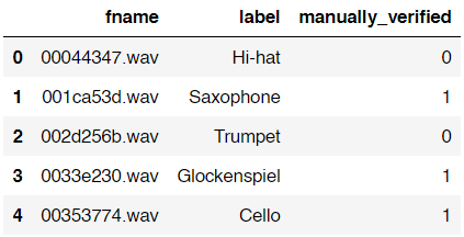
df.head()

Below is how the data frame looks like. You can see here that it contains filename-label pair and manually_verified column which I guess it’s used to tag whether an audio clip is verified by a real person.

As I’ve mentioned earlier, in this project I will only use 5 out of 41 classes in the dataset. Those classes are Cello, Saxophone, Acoustic_guitar, Double_bass and Clarinet. Here is how to filter out those classes.

df = df[df['label'].isin(['Cello','Saxophone','Acoustic_guitar','Double_bass', 'Clarinet'])]

Trending AI Articles:

1. Machine Learning Concepts Every Data Scientist Should Know

2. AI for CFD: byteLAKE’s approach (part3)

3. AI Fail: To Popularize and Scale Chatbots, We Need Better Data

4. Top 5 Jupyter Widgets to boost your productivity!

If you check the shape of the data you will find that the number of data is now only 1500 (previously there are 9473 files). As the data already filtered to only 5 classes, we will load those actual audio files using the following approach:

path = 'audio_train/'
audio_data = list()

for i in tqdm(range(df.shape[0])):
    audio_data.append(librosa.load(path+df['fname'].iloc[i]))

audio_data = np.array(audio_data)

Well, this process is relatively simple yet it takes several minutes to run. Here I declared an empty list called audio_data and append each of raw audio data using librosa.load() function. Keep in mind that the shape of this audio_data variable is (1500, 2) in which the first axis represents the number of raw audio waves and the second axis represents 2 columns (which stores audio waves and sample rate respectively). Lastly, I also convert the audio_data list into Numpy array.

By the way, if you use tqdm() function like what I did, you will have the output which looks something like this:

Now we will put the content of audio_data variable into data frame df which can be done using the following code:

df['audio_waves'] = audio_data[:,0]
df['samplerate'] = audio_data[:,1]
df.head()

Then it will show an output which looks like this:

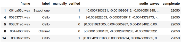
Our data frame with new column: audio_waves and samplerate.

Notice that the index number of the data frame is unordered. This is because we only take rows which contains the 5 labels I chose earlier. And fortunately for this case it’s completely fine to be like that.

Now, what I wanna do is to create 2 new columns which will store the length of each audio file, both in bits and seconds. Here is my approach:

bit_lengths = list()
for i in range(df.shape[0]):
    bit_lengths.append(len(df['audio_waves'].iloc[i]))

bit_lengths = np.array(bit_lengths)

df['bit_lengths'] = bit_lengths
df['seconds_length'] = df['bit_lengths']/df['samplerate']

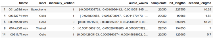
df.head()

I think the code above is pretty straightforward, I am sure you can understand it easily without further explanation.

Anyway, the two new columns are called bit_lengths and second_lengths. bit_lengths is essentially just the number of bits in each audio waves, while second_lengths is the length of all audio files in seconds. We can think of samplerate column like the number of frames in a video. Hence, in order to get the value for second_lengths, we can simply divide the number of all bits of each audio wave with the corresponding sample rate.

Now our data frame also contains the length of each audio file.

Step 2: Data generation

Up to this point, we already got a data frame df which now contains the length of all audio files. We just realized that actually all those audios are having different lengths. And well, this is a problem. Why? Because any machine learning or deep learning classifier models only accept data with exact same shape for each sample. So now, the solution is to make those data having the same length. In this project, I decided to go with 2 seconds of audio data.

In order to do it, the first thing I wanna do is to drop all samples which are shorter than 2 seconds. Here is the code to do it:

df = df[df['second_lengths'] >= 2.0]

Pretty simple isn’t it? Now if you check the number of data using df.shape, then you will have the shape of (1306, 7). You can see here that approximately 200 of our audio files are dropped thanks to this operation since those audios must be shorter than 2 seconds in length.

I use the code below to check whether we already eliminated audio files that have less than 2 seconds length.

min_bits = np.min(df['bit_lengths'])
print(min_bits)

min_seconds = np.min(df['second_lengths'])
print(min_seconds)

Both prints gives 44100 and 2.0 which represents the shortest audio file in the data frame in bits and seconds respectively.

We already done plenty of things as of this stage. Here I decided to make a checkpoint so that I don’t have to go through all those loadings if I want to run this code again in the future. So what I wanna do now is to utilize pickle module, which is very useful to store any kind of variables into separate file. And here in my case I want to store the data frame df into a file called audio_file.pickle. Below is the code for that.

with open('audio_df.pickle', 'wb') as f:
    pickle.dump(df, f)

Now assume that you’re now in the future and you want to reload the variable, you can do it simply by using the following code:

with open('audio_df.pickle', 'rb') as f:
    df = pickle.load(f)

That’s it! Now you got the exact same data frame (also stored in variable df) as what you saved in the past.

Anyway, that was just a way to create a checkpoint. If you feel like you don’t need one, just skip that part.

Okay, so actually I haven’t finished explaining about the entire part of data generation. Now what I wanna do next is to do what’s so-called as random sampling method — well, at least that’s how I call it.

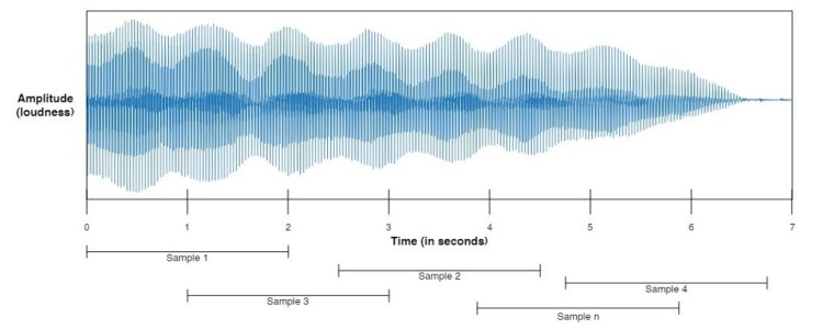
Data generation using random sampling method on audio waves.

So this random sampling works by taking n samples, where n is a number that we are free to choose. In this case, I want all those samples to have 2-seconds length. This 2-seconds audio chunk is taken at any position within an audio file in which the audio file itself is also selected randomly within the dataset for each iteration. Below is my implementation for this.

num_samples = 6000
generated_audio_waves = list()
generated_audio_labels = list()

for i in tqdm(range(num_samples)):
    try:
        chosen_file = np.random.choice(df['fname'].values)
        chosen_initial = np.random.choice(np.arange(0,df[df['fname']==chosen_file]['bit_lengths'].values-min_bits))
        generated_audio_waves.append(df[df['fname']==chosen_file]['audio_waves'].values[0][chosen_initial:chosen_initial+min_bits])
        
        generated_audio_labels.append(df[df['fname']==chosen_file]['label'].values)
    except ValueError:
        continue

generated_audio_waves = np.array(generated_audio_waves)
generated_audio_labels = np.array(generated_audio_labels)

Well, the point of the code above is to generate 2-seconds length audio in which it is stored in generated_audio_waves (for the wave data itself) and generated_audio_labels (for the labels of the corresponding wave data). Here I decided to take 6000 audio chunks which I declared using num_samples variable. Next, after generating all data, I also convert both lists to Numpy array because I think it’s just simpler than Python list.

Probably you might be wondering why I put try-except command in the code. And well, to be honest I completely got no idea why at certain iteration it always returns error. So, in order to handle that error, I just put a try-except command there and fortunately it only skips little number of data, which I think it doesn’t really affect the neural network model performance in the end.

Alright, I think I have to stop right now since I feel like this article has been very long. And, yea, this is the end of the first part of this project. I will continue explaining the next processes in part 2 (features preprocessing, label preprocessing, model training and model evaluation). See you there!