Semantic Segmentation for Pneumothorax Detection & Segmentation

So, Here in this Blog, i will show you that how can we solve the healthcare problem by enabling the power of Deep Learning.

Table of Contents:-

Introduction
Image Segmentation
Business Problem
Datasets
Prerequisites
Classification & Segmenatation Acrchitecture
Inference Pipeline
Conclusion
references

1. Introduction :

So here in this section we will discuss about computer vision,

https://machinelearningmastery.com/what-is-computer-vision/

Computer vision is the simply the process of perceiving the images and videos available in the digital formats.

In Machine Learning (ML) and AI — Computer vision is used to train the model recognize certain patterns and store the data into their artificial memory to utilize the same for predicting the results in real-life use

The application of computer vision in artificial intelligence is becoming unlimited and now expanded into emerging fields like automotive, healthcare, retail, robotics, agriculture, autonomous flaying like drones and manufacturing etc…

So here in this blog by enabling the power of deep learning , we will show you that how we can solve one of the problem of computer vision called ‘ Image Segmentation ’

2.Image Segmentation :

https://thegradient.pub/semantic-segmentation/

What is Image Segmentation?

Image Segmentation is a task of computer vision in which we partitioning images into different segments.

yes, sounds like Object detection , but no it different task than object detection …. Because Object Detection methods helps us draw bounding boxes around certain entities/Objects in Given Image ,

But on other side Image segmentation lets us achieve more detailed understanding of imagery than image classification or object detection.

in Simple words , in Image Segmentation we basically assign/classify each pixel to a particular class.

Types of Image Segmentation:

Semantic Segmentation
Instance Segmentation

https://www.kaggle.com/c/severstal-steel-defect-detection/discussion/108126

Semantic segmentation — classifies all the pixels of an image into meaningful classes of objects. These classes are “semantically interpretable” and correspond to real-world categories. For instance, you could isolate all the pixels associated with a cat and color them green. This is also known as dense prediction because it predicts the meaning of each pixel.

Instance segmentation — identifies each instance of each object in an image. It differs from semantic segmentation in that it doesn’t categorize every pixel. If there are three cars in an image, semantic segmentation classifies all the cars as one instance, while instance segmentation identifies each individual car.

Most Popular Chatbot Tutorials

1. Machine Learning Concepts Every Data Scientist Should Know

2. AI for CFD: byteLAKE’s approach (part3)

3. AI Fail: To Popularize and Scale Chatbots, We Need Better Data

4. Top 5 Jupyter Widgets to boost your productivity!

Application of Image Segmentation:

1 Medical Imagine

2 Computer Guided Surgery

3 Video surveillance

4 Recognition Tasks

5 Self-Driving Car

6 Industrial Machine Vision for product assembly and inspection

3. Business Problem :

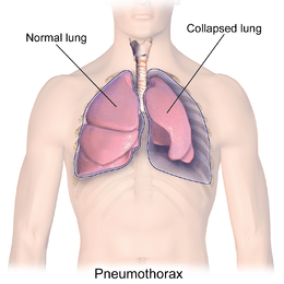
https://en.wikipedia.org/wiki/Pneumothorax

This Problem basically from the Healthcare domain. imagine suddenly
gasping for air, helplessly breathless for no apparent reason. Could it be a
collapsed lung? In the future, we are going to predict this answer.

Pneumothorax can be caused by chest injury, damage from underlying
lung disease, or most horrifying — it may occur for no obvious reason at all.
On some occasions, a collapsed lung can be a life-threatening event.

Pneumothorax is usually diagnosed by a radiologist on a chest x-ray
images ,but sometimes it could be difficult to confirm.

Pneumothorax is visually diagnosed by radiologist, and even for a
professional with years of experience; it is difficult to confirm.

So Our Goal is to Detect and Segment those Pneumothorax affected area with a help of Semantic Segmentation methods,so that we can help the radiologist by giving the results with higher precision.

Solution:

An AI algorithm to detect Pneumothorax would be useful to Solve this problem,

we will try to solve this problem in two Phase:

1 Pneumothorax Classification:

2 Pneumothorax Segmentation

So, in first phase we will develope a classification model to classify Pneumothorax and in Second Phase we will build a model for segmentaiton task on given image

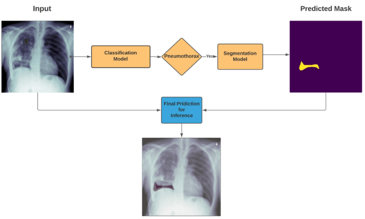
How prediction pipeline will work?

if Classification model detects the Pneumothorax in input X-Ray image then our Prediction Pipeline will pass that X-Ray image to Segmentation Model to segment the Pneumothorax in That X-ray image so that Radiology Expert can easily Analyze and Diagnose this Problem

This is How our Final Pipeline will Work

4. Dataset :

Before Going to Understand the Classification & Segmentation Architectures, let’s Have a glance at Dataset,

here we are using dataset which has been modified from the kaggle competition’s dataset.

so that we can easily get our input and target mask in (.png format).

Pneumothorax Dataset

4. Prerequisites :

Before start the Explaination Deep Learning Architecture, i assume that you have guys have a good Understanding of Basic Convolutional Operations like,

Conv2d, UpSampling , Dense Layers, Upconv2d Layer, Conv2dTranspose Layer , Softmax, Relu, BatchNormalisation all Basic stuff of Deep Learning with keras and most important Residual Block (ResNet & DenseNet).

5. Classification & Segmentation Architecture:

As you know that we have divided this problem into 2 part , So let’s have a look at part-1,

Part 1 : Pneumothorax Classification:

Basically here to solve this Classification problem , we have used DenseNet121 Architecture.

DenseNet:

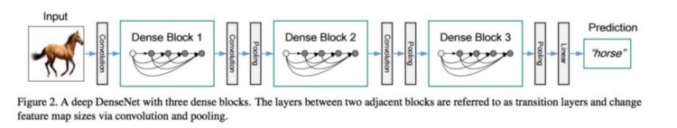
DenseNet is One of the new Architecute for image classification & Object Recognition , it is quite similar to ResNet Architecture with some fundamental differences, ResNet uses an additive method (+) that merges the previous layer (identity) with the future layer, whereas DenseNet concatenates (.) the output of the previous layer with the future layer.

Advantages of Densenet:

They alleviate the vanishing-gradient problem.
Strengthen feature propagation.
Encourage feature reuse.
Reduce the number of parameters.

here for our problem i used the DensNet-121 architecture Using this package,

from tensorflow.keras.applications.densenet import DenseNet121

But there is one more important thing that i have used to get state of the art results is, for Transfer Learning instead of using pre-trained weights of imagenet , i have used the weights of ChestXpert — DenseNet , because this ChestXpert model was trained on Medical X-Ray images to classify around 14 Disease which was related to Lungs.

and Pneumothorax was one of them so i directly loaded the weights of ChestXpert model for our DenseNet-121 but only for all convolutional blocks , and for dense layer i have initialized the weights using keras..

Below is the keras code to implement the above model,

from tensorflow.keras.applications.densenet import DenseNet121
from tensorflow.keras.layers import Dense, Input
from tensorflow.keras.models import Model, load_model

def get_chexnet_model():
  input_shape = (256, 256, 3)
  img_input = Input(shape=input_shape)
  base_weights = 'imagenet'

  #create the base pre-trained model
  base_model = DenseNet121(include_top=False,
                           input_tensor=img_input,
                           input_shape=input_shape,
                           weights=base_weights,
                           pooling='avg')

  x = base_model.output
  
  # add a logistic layer -- let's say we have 14 classes
  predictions = Dense(14,activation='sigmoid',name='predictions')(x)

  # this is the model we will use
  model = Model(inputs=img_input,
                outputs=predictions,)

  # load chexnet weights
  model.load_weights('/content/drive/My Drive/Case-Study    1/best_weights.h5')

  # return model
  return base_model, model

tf.random.set_seed(1234)
base, model = get_chexnet_model()
x = Dense(1024, activation='relu', kernel_initializer='he_normal')(model.layers[-2].output)
x = Dense(2, activation='softmax', kernel_initializer='he_normal')(x)

final_model =  Model(model.input, x)
final_model.summary()

and you if you guys want to Understand the DenseNet Architechure then Must read this Paper on DenseNet architecture

Training:

To Train this model we used

final_model.compile(optimizer='adam', loss='categorical_crossentropy', metrics=[tf.keras.metrics.AUC(), 'accuracy'])

final_model.fit_generator(generator=Train_pipeline, epochs=30, validation_data=Test_pipeline)

and we achieved 90%Accuracy on trainset and 87% Accuracy on validation set….

So now after completing the part 1 ,Let’s have a look at Part -2

Part 2: Pneumothorax Segmentation:

Now we will discuss most important part of this blog ,

For this task we have implemented the Architecture called ” UNet++ : nested UNet architecture” , it is the advanced or can say extended version of UNet.

to Understand this architecture must have basic idea about how UNet work for Semantic segmentation , you can read this to understand the UNet Architecture.

So i hope now you will have a better understandings of UNet.

UNet++ : Nested UNet architecture for Medical Image Segmentaion:

So as you can see in this diagram so we will find some similarites between UNet and UNet++

Because Like Unet , UNet++ also follows the same encoder-decoder approch to generate the semantic segmentation

But here i have mentioned some points which differs UNet++ from UNet:

Convolution layer on skip pathways which bridges the semantic gap between encoder-decoder
Dense skip connections at skip pahways which improves the Gradient flow and prevents from gradient vanishing problem
Deep Supervision which improves the model pruning

that’s it , But if you want to go more deeper to understand How this things work in UNet++ then you from here you will get the better idea

Below keras code will help you to define above model (UNet++):

def convolution_block(x,filters,\
                      size,strides(1,1),\ 
                      padding='same',activation=True):
 x = BatchNormalization()(x)
 if activation == True:
  x = LeakyReLU(alpha=0.1)(x)
 return x


def residual_block(blockInput, num_filters=16):
  x = LeakyReLU(alpha=0.1)(blockInput)
  x = BatchNormalization()(x)
  blockInput = BatchNormalization()(blockInput)
  x = convolution_block(x, num_filters, (3,3) )
  x = convolution_block(x, num_filters, (3,3), activation=False)
  x = Add()([x, blockInput])
  return x

from efficientnet import EfficientNetB4

def UEfficientNet(input_shape=(None, None, 3),dropout_rate=0.1):
  backbone = EfficientNetB4(weights='imagenet',\
                              include_top=False,\
                              input_shape=input_shape)
  input = backbone.input
  start_neurons = 8

  conv4 = backbone.layers[342].output
  conv4 = LeakyReLU(alpha=0.1)(conv4)
  pool4 = MaxPooling2D((2, 2))(conv4)
  pool4 = Dropout(dropout_rate)(pool4)
  
  # Middle
  convm = Conv2D(start_neurons * 32, (3, 3), activation=None,\
                 padding="same",name='conv_middle')(pool4)

  convm = residual_block(convm,start_neurons * 32)
  convm = residual_block(convm,start_neurons * 32)
  convm = LeakyReLU(alpha=0.1)(convm)
 
  deconv4 = Conv2DTranspose(start_neurons * 16, (3, 3), strides=(2,   2), padding="same")(convm)
  deconv4_up1 = Conv2DTranspose(start_neurons * 16, (3, 3), strides=(2, 2), padding="same")(deconv4)
  deconv4_up2 = Conv2DTranspose(start_neurons * 16, (3, 3), strides=(2, 2), padding="same")(deconv4_up1)
  deconv4_up3 = Conv2DTranspose(start_neurons * 16, (3, 3), strides=(2, 2), padding="same")(deconv4_up2)

  uconv4 = concatenate([deconv4, conv4])
  uconv4 = Dropout(dropout_rate)(uconv4)
  uconv4 = Conv2D(start_neurons * 16, (3, 3), activation=None, padding="same")(uconv4)
  uconv4 = residual_block(uconv4,start_neurons * 16)
  uconv4 = LeakyReLU(alpha=0.1)(uconv4)  #conv1_2

  deconv3 = Conv2DTranspose(start_neurons * 8, (3, 3), strides=(2, 2), padding="same")(uconv4)

  deconv3_up1 = Conv2DTranspose(start_neurons * 8, (3, 3), strides=(2, 2), padding="same")(deconv3)

  deconv3_up2 = Conv2DTranspose(start_neurons * 8, (3, 3), strides=(2, 2), padding="same")(deconv3_up1)

  conv3 = backbone.layers[154].output
 
  uconv3 = concatenate([deconv3,deconv4_up1, conv3])
  uconv3 = Dropout(dropout_rate)(uconv3)
  uconv3 = Conv2D(start_neurons * 8, (3, 3), activation=None,  padding="same")(uconv3)
  uconv3 = residual_block(uconv3,start_neurons * 8)
  uconv3 = LeakyReLU(alpha=0.1)(uconv3)
 
  deconv2 = Conv2DTranspose(start_neurons * 4, (3, 3), strides=(2, 2), padding="same")(uconv3)
  deconv2_up1 = Conv2DTranspose(start_neurons * 4, (3, 3), strides=(2, 2), padding="same")(deconv2)

  conv2 = backbone.layers[92].output
  uconv2 = concatenate([deconv2,deconv3_up1,deconv4_up2, conv2])
  uconv2 = Dropout(0.1)(uconv2)
  uconv2 = Conv2D(start_neurons * 4, (3, 3), activation=None, padding="same")(uconv2)
  uconv2 = residual_block(uconv2,start_neurons * 4)
  uconv2 = LeakyReLU(alpha=0.1)(uconv2)
  
  deconv1 = Conv2DTranspose(start_neurons * 2, (3, 3), strides=(2, 2), padding="same")(uconv2)
  conv1 = backbone.layers[30].output
  uconv1 = concatenate([deconv1,deconv2_up1,deconv3_up2,deconv4_up3, conv1])
  uconv1 = Dropout(0.1)(uconv1)
  uconv1 = Conv2D(start_neurons * 2, (3, 3), activation=None, padding="same")(uconv1)
  uconv1 = residual_block(uconv1,start_neurons * 2)
  uconv1 = LeakyReLU(alpha=0.1)(uconv1)
  uconv0 = Conv2DTranspose(start_neurons * 1, (3, 3), strides=(2, 2), padding="same")(uconv1)
  uconv0 = Dropout(0.1)(uconv0)
  uconv0 = Conv2D(start_neurons * 1, (3, 3), activation=None, padding="same")(uconv0)
  uconv0 = residual_block(uconv0,start_neurons * 1)
  uconv0 = LeakyReLU(alpha=0.1)(uconv0)
  uconv0 = Dropout(dropout_rate/2)(uconv0)

  output_layer = Conv2D(1, (1,1), padding="same",   activation="sigmoid")(uconv0)
  
 model = Model(input, output_layer)
 model.name = 'u-xception'
 return model

tf.keras.backend.clear_session()

img_size = 256
model = UEfficientNet(input_shape=(img_size,img_size,3),dropout_rate=0.3)

Training:

To train this model , I used

Dice_Loss:

Generally for image segementation task , combination of binary cross_entropy and Dice_loss is being used immensely ,

because as we all know only binary cross entropy is not good option while you will having an imbalanced dataset , but here this Dice_loss works excellenty in those scenario ,

so our final loss will be

loss function = Binary_crossentropy + Dice_Loss, where N=Batch_size

IoU_Score (Intersection over Union):

so we have talked about loss, but what about Evaluation Metrics, should we use Accuracy ???

so Answer is No, for Image Segmenation or Object Localization task IoU_score is being Used extensively ,

Basically Accuracy function will also take those region/pixels which is not part of that object in specific image , specially for medical image segmentation task in which targeted mask contains very less amount of pixel , so in that case accuracy will always be high without taking care about location of the affected region by disease,

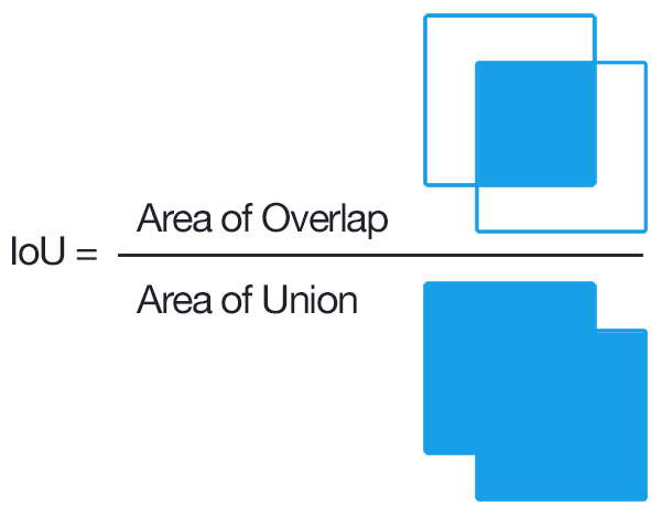
https://www.pyimagesearch.com/2016/11/07/intersection-over-union-iou-for-object-detection/

after looking at this diagram , you would have get the idea about how IoU Score works ,

It comes in handy when you’re measuring how close an annotation or test output lines up with the ground truth. As a ratio of the areas of intersection and union, it works on annotations of all shapes and size.

What’s cool is how IOU can be used with F1 scores to measure the accuracy of object detection tasks with multiple annotations per image

so after set the loss and evaluation matrice , we train this model using adam as an optimiser for 40 epochs,

so after 40 epochs of training we were able to get 0.73 IoU_Score and 0.71 val_IoU_Score.

7. Inference Pipeline:-

So as I mentioned in earlier in Inference pipeline’s Diagram ,

we will only predict the segmentation mask for input Chest X-Ray image if our Classifier will detects any Pneumothorax in that X-ray Image, otherwise there is no mean to predict the segmentation mask for that

here i am showing some predictions of our segmentation model…

Green: Groundtruth mask Red: Predicted mask

Here, Green Pixels Represents the Groundtruth (Actual Mask) & Red Pixels Represents the Predicted Mask.

we we have developed the complete Class called Pipeline for final production pipeline.

class Pipeline():
   
   def __init__(self, segmentation, classifier):
     self.segmentation = segmentation
     self.classifier   = classifier
   
   def Predict(self, ix):
     image = cv2.imread(mask_df.loc[ix, 'image'])
     img_clf = image/255.0
     pre_cls  =np.argmax(self.classifier.predict(tf.expand_dims(img_clf, axis=0), steps=1))
     plt.imshow(image)
     
    if pre_cls==1:
      img_seg = self.segmentation.predict(tf.expand_dims(image, axis=0), steps=1) 
      plt.imshow(img_seg[0,:,:,0], cmap='Reds', alpha = 0.4)
      plt.title("Pneumothorax is Detected.........")

    else:
      plt.title("Pneumothorax is not Detected.........")
    plt.show()

So our pipeline will segment the predicted mask by presenting it in red region , which will show the location of Pneumothorax in given input X-Ray image of Patient

8. Conclusion :-

i really appreciate you for giving time to read this blog

so please clap it if you like and learn new things from this blog , because it will encourage me to share more knowledge and informations related to Deep Learning through my blogs.

Thank You.