
Non-Negative Matrix Factorization for Dimensionality Reduction
We have explained how we can reduce the dimensions by applying the following algorithms:
We will see how we can also apply Dimensionality Reduction by applying Non-Negative Matrix Factorization. We will work with the Eurovision 2016 dataset as what we did in the Hierarchical Clustering post.
Few Words About Non-Negative Matrix Factorization
This is a very strong algorithm which many applications. For example, it can be applied for Recommender Systems, for Collaborative Filtering for topic modelling and for dimensionality reduction.
In Python, it can work with sparse matrix where the only restriction is that the values should be non-negative.
The logic for Dimensionality Reduction is to take our m x n data and to decompose it into two matrices of m x features and features x n respectively. The features will be the reduced dimensions.

Dimensionality Reduction in Eurovision Data
Load and Reshape the Data
In our dataset, the rows will be referred to the Countries that voted and the columns will be the countries that have been voted. The values will refer to the ‘televote’ ranking.
import pandas as pd
import numpy as np
import matplotlib.pyplot as plt
%matplotlib inline
eurovision = pd.read_csv("eurovision-2016.csv")
televote_Rank = eurovision.pivot(index='From country', columns='To country', values='Televote Rank')
# fill NAs by min per country televote_Rank.fillna(televote_Rank.min(), inplace=True)
The televote_Rank.shape is (42, 26)
Non-Negative Matrix Factorization
Since we have the data in the right form, we are ready to run the NNMF algorithm. We will choose two components because our goal is to reduce the dimensions into 2.
# Import NMF from sklearn.decomposition import NMF
# Create an NMF instance: model
model = NMF(n_components=2)
# Fit the model to televote_Rank
model.fit(televote_Rank)
# Transform the televote_Rank: nmf_features
nmf_features = model.transform(televote_Rank)
# Print the NMF features
print(nmf_features.shape)
print(model.components_.shape)
As we can see we created two matrices of (42,2) and (2,26) dimensions respectively. Our two dimensions are the (42,2) matrix.
Trending AI Articles:
1. Microsoft Azure Machine Learning x Udacity — Lesson 4 Notes
2. Fundamentals of AI, ML and Deep Learning for Product Managers
Plot the 42 Countries in two Dimensions
Let’s see how the scatter plot of the 42 countries into two dimensions.
plt.figure(figsize=(20,12))
countries = np.array(televote_Rank.index)
xs = nmf_features[:,0]
ys = nmf_features[:,1]
# Scatter plot plt.scatter(xs, ys, alpha=0.5)
# Annotate the points
for x, y, countries in zip(xs, ys,countries):
    plt.annotate(countries, (x, y), fontsize=10, alpha=0.5) plt.show()
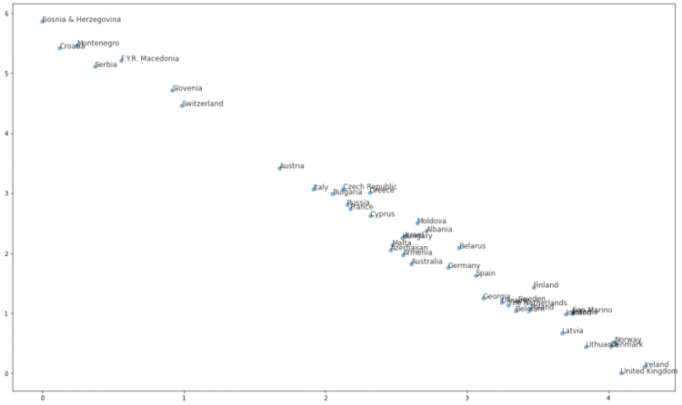
Can you see a pattern?
The 2D graph here is somehow consistent with the dendrogram that we got by applying the linkage distance. Again, we can see a “cluster” of the cluster from “ Yugoslavia” and also that the Baltic countries are close as well as the Scandinavian and the countries of the United Kingdom.
Don’t forget to give us your ? !


Non-Negative Matrix Factorization for Dimensionality Reduction — Predictive Hacks was originally published in Becoming Human: Artificial Intelligence Magazine on Medium, where people are continuing the conversation by highlighting and responding to this story.
