Equipment Failure prediction Using ML: for Stripper Wells

Here in this blog, how you can leverage an application of Data science & Machine learning in Oil Industry

1. Introduction
2. Business Problem
3. ML formulation
4. Business Constraint
5. Dataset
6. Performance Metric
7. EDA
8. ML modeling
9. Custom Ensemble Classifier (Stacking)
10. Future work
11. Conclusion
12. References

1. Introduction:-

what is Stripper Well ?

Stripper well is mechanical equipment , which is used for oil mining , it is entry level well property which does not exceed the specific amount of barrels of oil in oil mining industry and due to it’s low capacity of production in oil mining , it is near to the end of its economical application in industry, but in present it is widely adopted in US oil mine Industry

2. Business problem:-

Stripper wells are very cheap and companies have been using it since very long time, and it Might get expensive to implement new well technology to produce larger amount of oil from mining,

but it is mechanical property so industries have to maintain it every year and they have to fix all mechanical failures that comes within those strippers well, otherwise, it may causes money losses in oil production,

and when these kind of failure occurs, oil prices can go higher….That’s why it becomes mandatory to find and fix these mechanical equipment failure as soon as possible, but again it requires expertise in finding the process of equipment failure,

“ but what if we can detect these equipment failures by enabling the power of machine learning?? “

3. ML Formulation:-

Our problem is to find equipment failure in stripper well with help of machine learning,

Yes, we can solve this issue by predicting surface and down-hole failure in equipment and save the amount of time that can wasted in to detecting process of failure in manual way, and after the prediction of equipment failure, engineers can fix the equipment on surface or send the workout rig to well location to pull out the down-hole equipment so that engineers can fix it on surface level.

4. Business Constraint:-

As machine learning prediction pipeline will going to be implemented on well using sensors ,

failure will be going to be predicted using these ML pipeline by getting input data from sensors ,

So that, field engineers will be able to monitor the equipment failure whenever they want, due to this implementation strategy we can figure out that our ML pipeline should be capable enough to predict a failure within the few seconds or maybe in 1–2 mins , then we will be able to address this failure issue as soon as possible

Trending AI Articles:

1. Microsoft Azure Machine Learning x Udacity — Lesson 4 Notes

2. Fundamentals of AI, ML and Deep Learning for Product Managers

3. Roadmap to Data Science

4. Work on Artificial Intelligence Projects

5. Dataset:-

Basically, Dataset that we have chosen to solve this problem contains 109 columns

1) Id: which is Unique id number for each sensor’s input.

2) Target: in this column label has been given given for equipment failure ,if 0 then “ no failure ” and if 1 then “failure occured”.

3) There are two types of sensor columns:

Measure columns: these columns are single measurement for the sensor.

Histogram bin columns: These are set of 10 columns that are different bins of a sensor that show its distribution over time

6. Performance Matrix:-

As we are posing our problem as Binary Classification problem ,

We will use 1) micros f1-score to measure the performance of our model’s prediction

7. EDA:

Here we have reached at the most important part of our Case Study EDA, in this section, we will discussed about how we have done the Exploratory Data Analysis on Our Data,

1 Class Imbalanced :

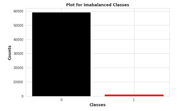
Here in this class imbalaced plot, we can clearly notice that classes are highly imbalanced , we have only 1000 positive datapoints which carries the data values when the equipment failure was occured, so we know that machine learning model becomes easily biased and produce very low recall value for minority class when we carries the class imabalaced problem in our dataset

2. Data Cleaning:

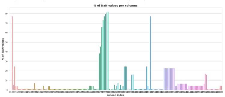
this plot shows the percentage of Nan value in each column , it is clear that there are plenty of Nan values in our dataset, and there are almost 24–25 columns which carries more than 20% of Nan values, so we have find out a way to get rid of these Nan values.

there is one of the most basic solution is to drop the columns which carries atleast one Nan value , but applyting that operation we just left with only 593 raws out of 60,000 , which means there are only 1% raw which does not have any Nan-value, so that it may lead us towards the very high data-loss

That’s why we have to find the optimal threshold percentage value by looking at this plot, so that we remove those columns which carries Nan-value percentage more than that choosen threshold and replace the Nan-value with constants in rest of other columns, But..

But how can we select that threshold ??

Here, we have selected some threshold values like [5,10,20,30,40,50,60,70,80] using which we are going to perform some experiments on data to check how dropping of Nan-value affects on

1) Class Distribution

2) Dimensionality of Data

but you will ask why did i selected the 80 as maximum because there are few columns which has Nan-values between 80–85%.

so here in this plot annotation of each scatter point suggests the threshold value that we have selected for dropping the columns and after dropping those columns which contains Nan value more than the percentage of that annoted threshold ,

we dropped all rows which carries at least 1 Nan value , because previously we have seen that if we directly drops the rows then we are loosing 99% of datapoints because of some columns which carries more than 50% of Nan values within it’s, so that first we have dropped those columns and then we dropped the rows to check whether it is affecting on class imbalance issue or not

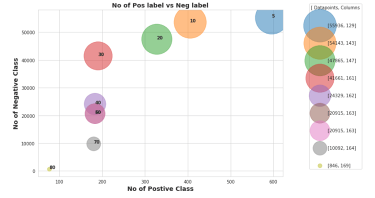
in this plot, we can analyze that if we first drops the columns using 80% as threshold , then we are getting rid from the class imbalanced problem but we only lefts with the 846 datapoints with 164 columns , which may cause the curse dimentionality issue in model training so it is not good threshold value,

and we choose 5% as threshold then it clear that we won’t have to face datapoints loss , because with 5% we will have ~56,000 datapoints but , if you have noticed or not but we lost the almost 129 columns and classes are also highly imbalanced by selecting 5% we are loosing around 400 datapoints from class-1(positive) , which is also not preferred value to drop the columns

so after spending some time on selecting optimal threshold value to dropped the Columns, i found that 20% as a threshold as which we had selected in previous

after selecting the threshold we have dropped the columns which was carrying more than 20% of Nan values, and

then we will impute the constant in rest of Nan values based on it’s column mean or median values.

3. Feature Selection:

for feature selection i used Phi_k feature correlation metric to check the correlation of input variables with the target variable

Above Heatmap shows the Phi_K matrix, but we can’t analyze, how much columns should we select by just looking at this heatmp, but yeah we can say we some points in first columns which shows more than 50 of correlation value with targeted column

So we have plotted the Barplot to Analyze and select the best features those are highly correlated with the Target Column

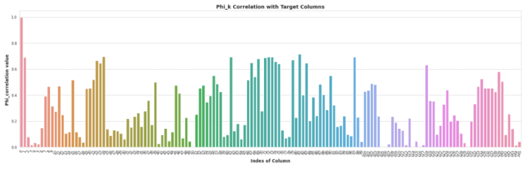
in Phi_k Correlation Method column is highly Correlative when it Phi_k correlation value is near to 1 and less Correlative when it nears to 0.

here we also wanted to select top 15 columns based on the phi_k correlation with target columns but if we choose 15 then it might have a chance that not a any single columns would be seleted from histogram_bin’s column set,

therefore we are going select top 30 columns based on them phi_k correlation score with target column

4. Univariate Analysis:-

here we have selected top 30 features based on it’s phi_k correlation score now it’s time to check how these features are distributed

so to check this we have plotted violin plot for each columns so that we can analyze the distribution of the columns

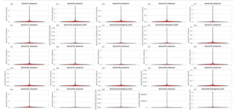
In these plot we can see the violin plots for each feature column, and we have noticed one thing that each column contains the some amount of outliers, that we have detect and remove specially if it is from negative class, because number of points in Negative class is very high as compare to the Positive class, and if we toss the dataset for training with ouliers especially from the Negative class then Prediction model will become biased the Mejority class(in our case Negative Class)

therefore, further try to detect and remove the outliers of the Negative class and we will put as it is the positive class’s outliers because it will help use to make model equally biased for both classes

5. Detect Remove Outliers:

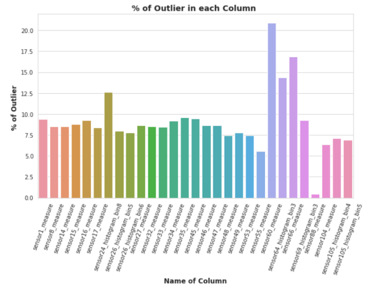
So Here in above plot it’s clear that almost all columns have outliers and most of them carries more than 5% of outliers. so if we will remove these outlier points then we might have to face loss of datapoint and will have less than 1000 of datapoints out of 60000 datapoints, and it will also increased class imbalanced problem,if it removes the outlier of minority class(Positive) then

so, we can do one thing in, future when we will start to developing a model for prediciton at that time we have to do undersampling on majority class which is negative class in our case, so somehow it will alliviate the problem of outliers and class imbalance,therefore we will remove the outliers of only negative class so that it will decreased the number of negative class points

Shape of Final :  (31131, 30)
Class-Distribution:
 0.0    30131
1.0     1000
Name: target, dtype: int64

After removing the outliers from the negative class , we can see that the number of datapoints of negative class has decreased from 59,000 to 34,735.

8. ML Modelling:-

Performance Metric: F1-Score(Micro): so to select best model we will use F1 score (micro) because ‘micros’ Calculate metrics globally by counting the total true positives, false negatives and false positives, and for our problem false positives and false positives matters a lot so instead of taking simple f1-score, we choose this as KPI metric for our problem

here we will train 6 different models and will find best hyperparameters by train and testing the model on cv-set using Linear Search , And then we will train these model using that tuned hyperparameter and after these trained model we will calculate the micro F1-score of test data and then we will compare the best result and select the best model which will give the highest micro F1-score on Test data

Models that we are going to train for this Experiments:

1. Random (For findng the worst case)
2. Logistic Regression
3. KNN
4. SVM(Linear)
5. SVM(RBF)
6. Decision Tree Classifier
7. Random-Forest (ensemble)
8. Gradient Boosting (Boosting)

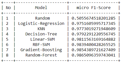
So, after completion of the various Machine Learning model’s training. we can conlude that the Random-Forest is best model among the other models which has achieved micro F1-Score = 0.9854 on Test Data after Tuning with the “n_estimator” hyperparameter on cross-validation set.

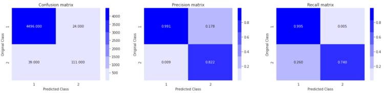
Result the we get on Test Data with our Best model

9. Custom Ensemble Classifier (Stacking):-

Even of having such a good results , we tried one new approach to get better results

here to train this Custom Ensemble Classifier ,

we followed these steps

1) First we have Split your whole data into train and test(80–20)

2) then in the 80% train set, again we split the train set into D1 and D2.(50–50).

then we did sampling with replacement from D1 to create d1,d2,d3….dk(k samples)

after that we created ‘k’ models and trained each of these models with each of these k samples.

3) so after done with training of k model , we passed the D2 set to each of these k models, and then we get k predictions for D2, from each of these models.

4) after it using these k predictions we created a new dataset, and for D2, and as we already know it’s corresponding target values, so then we trained a meta model with these k predictions by considering it as a meta data.

5) and for model evaluation, we have used the 20% data that we have kept as the test set. Passed that test set to each of the base models and we got ‘k’ predictions. after that we created a new dataset with these k predictions and passed it to meta-model

and we got the final prediction. Then using this final prediction as well as the targets for the test set, we have calculated the models performance score.

To get more insights about this approach ,you can check this paper:

https://pdfs.semanticscholar.org/449e/7116d7e2cff37b4d3b1357a23953231b4709.pdf

Here, in this Custom Stacking model ,

1. Base k Leaner : we used Decision Tree classifer with higher “max_depth”
2. Meta Model : Random Forest Classifer (with n_estimator=k)

we had K (number of base learner as a Hyper parameter & n_esimator of random forest (meta-model))

So to pick best number of k ,we did Gridsearch using different values([5, 10, 50, 100, 200, 500, 1000]) of K and then compare the results that we have calculated on test set

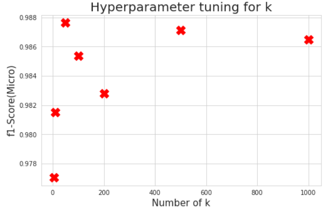
here we can see that we have achieved micro f1-score ~0.9880 with k=50, so now we are going to train our model with k=50.

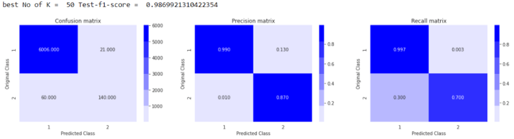
here, you can notice that we have achieved better results then using only just Randomforest Classifier ,

because of having good Precision and Recall we have finalized this Custom Stacking Classifier

10. Inference Pipeline:

So for inference Pipeline we will take the input from only selected sensor’s data which we have selected using Feature Selection

Above we have given Inference pipeline’s code, you can visit this from “Code for inference pipeline “ , or you guys can visit my GitHub repository for this project from where you can get it

10. Future Work:-

So to Carry this project For more batter results, you can train NN instead of using Custom Stacking Classifier or You can Combine both of this

and for more Advanced approach, you can Trained RNN, LSTM based Classifier using Only Histogram bin’s Columns from our Dataset.

11. Conclusion:-

after looking at these results of the inference pipeline, for industry purpose this pipeline can be installed at the onside Computers or maybe on cloud. Next industry operator or Engineers can connect the sensors with IoT devices to get the reading from sensors and then they can monitor the health of the stripper wells periodically by looking at the predictions of that readings, which will be collected through Sensors

12.references:-

Custom Stacking Classifier Paper:- https://pdfs.semanticscholar.org/449e/7116d7e2cff37b4d3b1357a23953231b4709.pdf

You can get Code from here:

GitHub: https://github.com/smit8800/Equipment-Failure-prediction-Using-ML-for-Stripper-Wells

LinkedIn: https://www.linkedin.com/in/smit-kumbhani-44b07615a

Don’t forget to give us your ? !

---

Equipment Failure prediction Using ML: for Stripper Wells was originally published in Becoming Human: Artificial Intelligence Magazine on Medium, where people are continuing the conversation by highlighting and responding to this story.

Via https://becominghuman.ai/equipment-failure-prediction-using-ml-for-stripper-wells-6f973aff3070?source=rss—-5e5bef33608a—4