
How to evaluate Machine Learning models? — Part 1
Before getting deep into artificial intelligence, it is important to understand which model should deploy? what are the metrics with respect to dataset and the application of model.
Like a Teacher with the model as our students, there are some parameters or we can say benchmark — decides the quality of our model whether the given model will be selected or it will be rejected.
Below is the brief classification of the metrics which we will be discussing in this as well as the upcoming part.
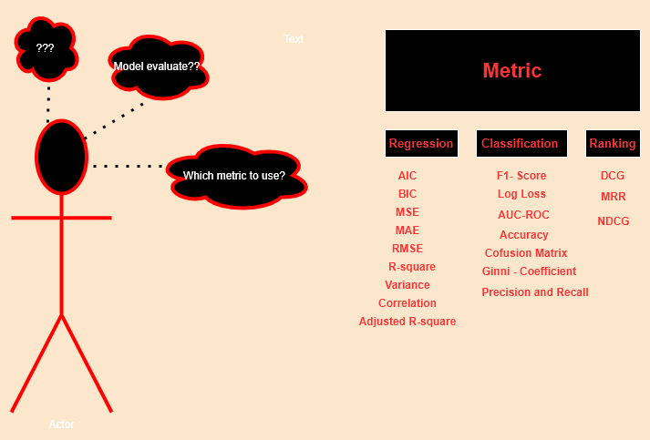
In this part i.e. part 1 we are going to cover varoius metrics. So without any further delay lets start.
Before boarding, let assume that we have trained one regression model whose name is Learned_Model and after training it gives output as “O” (predicted)for n sample and for “n” number of sample it gives n*O, whereas we have actual output denoted as “Y”(target variable) for n sample,

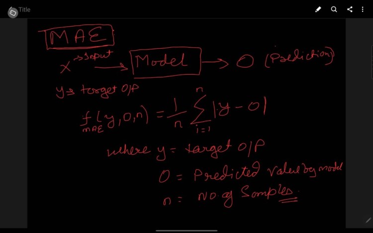
1. MAE (Mean Absolute Error)
MAE is we break this we will have three separate words i.e. Error, Absolute, and Mean (traversing right to left) where,
Error is the difference between the target and predicted value i.e. Y-O
Absolute is defined as the absolute value of the error i.e. |Y-O|, let it be AE
Mean is defined as taking the average of the Absolute error for n sample
i.e ∑ AE /n(AE), where n(AE) is number of sample i.e. n.
Link for code: jupyter notebook
2. MSE (Mean Square Error)
Similarly, if we break MSE this we will have three separate words i.e. Error, Square, and Mean (traversing right to left) where,
Error is the difference between the target and predicted value i.e. Y-O
Absolute is defined as the absolute value of the error i.e. (Y-O)², let it be SE
Mean is defined as taking the average of the Absolute error for n sample
i.e ∑ SE/n(SE), where n(SE) is number of sample i.e. n.
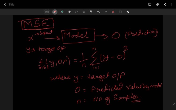
Note MAE in robust to the outlier than MSE because by squaring the error, the outliers — a high error that other samples get more attention and dominance in the final error hence impact the model parameters.
Link for code: jupyter notebook
Trending AI Articles:
1. Fundamentals of AI, ML and Deep Learning for Product Managers
3. Graph Neural Network for 3D Object Detection in a Point Cloud
4. Know the biggest Notable difference between AI vs. Machine Learning
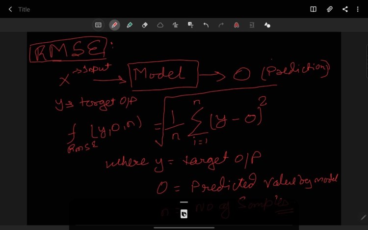
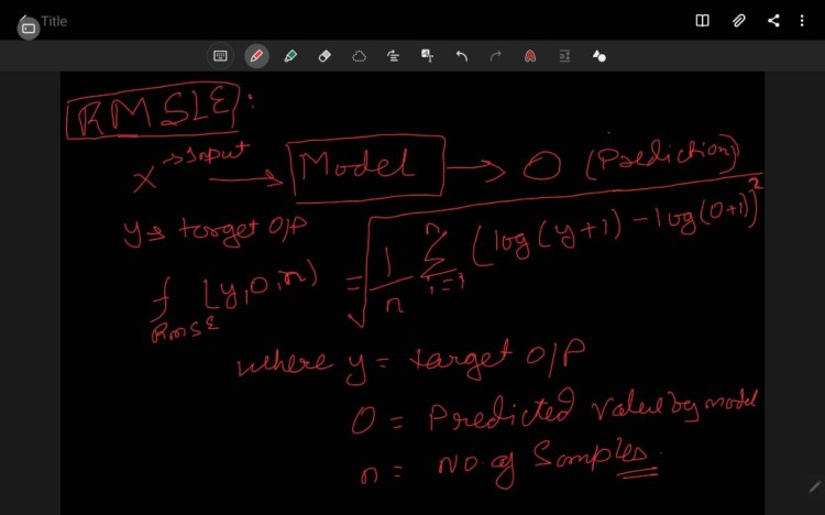
3. RMSE (Root Mean Square Error)
Similarly, if we break RMSE this we will have three separate words i.e. Error, Square, Mean, and Root (traversing right to left) where,
Error is the difference between the target and predicted value i.e. Y-O
Absolute is defined as the absolute value of the error i.e. (Y-O)², let it be SE
Mean is defined as taking the average of the Absolute error for n sample
i.e ∑ SE/n(SE), where n(SE) is number of sample i.e. n.
The root is defined as taking the root of the MSE i.e ( ∑ SE/n(SE))^(1/2)
RMSE is highly affected by outliers. In RMSE the power of root empowers it to show a large no. of deviations. As compared to MAE, RMSE gives higher weightage and punishes large errors.
RMSLE denotes Root Mean Square Logarithm Error a derivative of RMSE which scale down the error. Basically it is used when we don’t want to penalize the huge difference in the predicted (Y) and the target value(O), when the predicted value (O) is True Positive i.e. correct.
If both O and Y values are small: RMSE == RMSLE
If either O and Y values are big: RMSE >RMSLE
If both O and Y values are big: RMSE >RMSLE — almost negligible.
Link for code: jupyter notebook
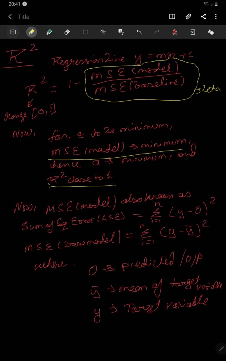
4. R² (R-squared)
R² is also known as the coefficient of determination used to determine the goodness of fit I .e.shows how well the model fits the line or shows how data fit the regression model. Basically it determines the proportion of variance in the D.V that can be explained by I.V. Generally higher the value of R² better the model performs but in some cases this thumb rule also fails to validate. So, we need to consider the other factors also along with the R².
In simple words, we can say how good is our model when compared to the model which just predicts the mean value of the target from the test set as predictions.
Link for code: jupyter notebook
5. Adjusted R²
As we have discussed R² above, similarly Adjusted R² is an improvised version of the R².
R² is biased it means if we add new features or I.V if does not penalize the model respective of the correlation of the I.V. It always increases or remains the same i.e. no penalization for uncorrelated I.V.

In order to counter this problem of non-decrement of R² value, a penalizing factor has been introduced which penalizes the R².
Theoretical intuition of Adjusted R² refer below image:

Mathematical intuition of Adjusted R² refer below image:

Link for code: jupyter notebook
6. Variance
In Decision trees, the inverse variance is defined by the homogeneity of the node i.e. less the variance more the homogeneity, and hence purity of the node is increased. Variance is used to decide the split of the node which has continuous samples.
The larger the spread of the tail larger the dispersion hence variance is large in terms of Normal Distribution.
For formulae refer to the image.

Link for code: jupyter notebook
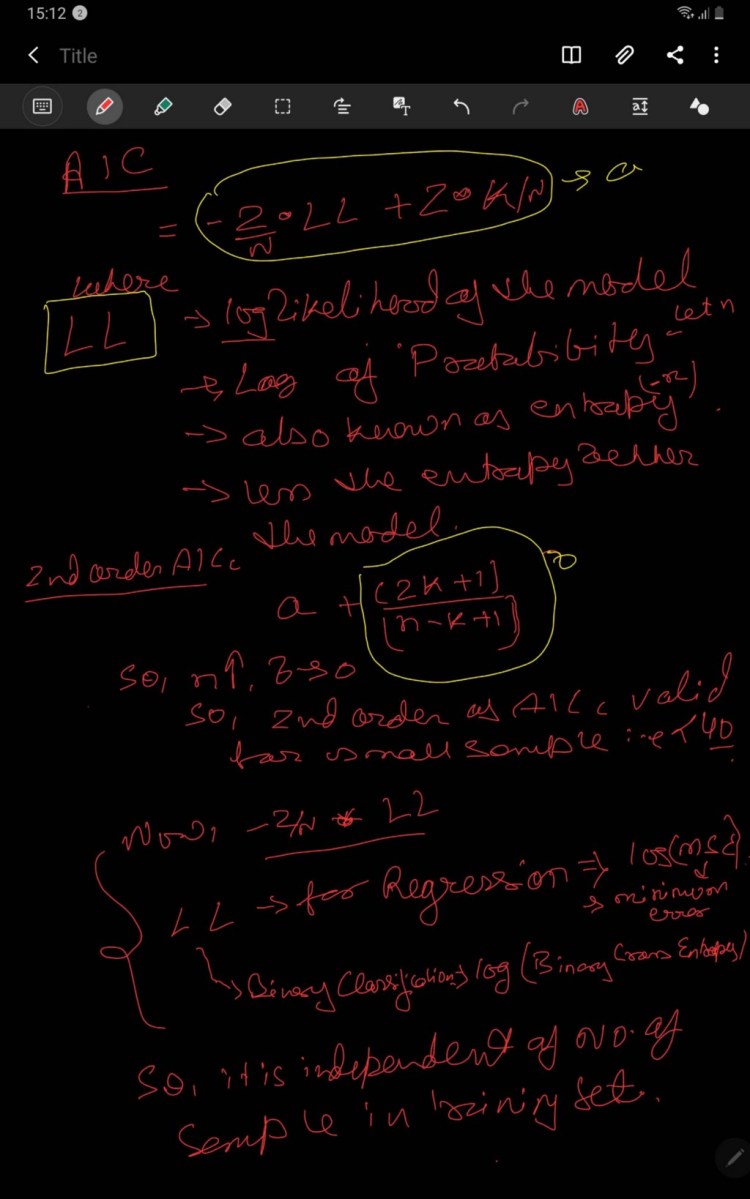
7. AIC
AIC refers to Akaike Information Centre is a method for scoring and selecting a model, developed by Hirotugu Akaike.
AIC shows the relationship between Kullback-Leibler measurement and the likelihood estimation of the model. It penalizes the complex model less i.e. it emphasize more on the training dataset by penalizing the model with an increase in the IV. AIC selects the complex model, the lower the value of AIC better the model.
AIC= -2/N *LL + 2*k/N, where
N= No. of Samples in training,
LL=LogLikelihood of model
K= no. of parameters in training dataset.
For mathematical explanation refer to this image.
Link for code: jupyter notebook
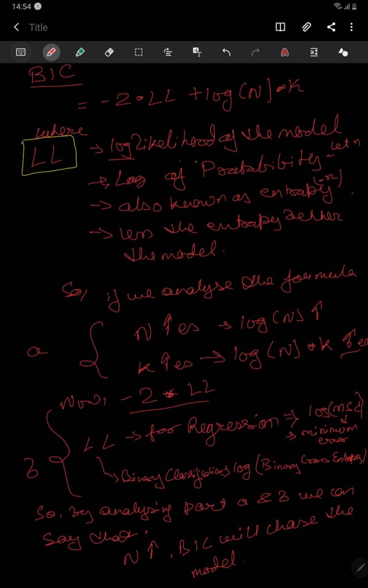
8. BIC
BIC is a variant of AIC known as Bayesian Information Criterion. Unlike the BIC, it penalizes the model for its complexity and hence selects the simple model. The complexity of the model increases, BIC increases hence the chance of the selection decreases.
BIC = -2 * LL + log(N)*k, where
k= no. of parameters,
LL= logLikelihood,
N= No of sample in training dataset.
For mathematical explanation refer to this image.
Special Thanks:
As we say “Car is useless if it doesn’t have a good engine” similarly student is useless without proper guidance and motivation. I will like to thank my Guru as well as my Idol “Dr P. Supraja”- guided me throughout the journey, from bottom of my heart. As a Guru, she has lighted the best available path for me, motivated me whenever I encountered failure or roadblock- without her support and motivation this was an impossible task for me.
Contact me:
If you have any query feel free to contact me on any of the below-mentioned options:
Website: www.rstiwari.com
Google Form: https://forms.gle/mhDYQKQJKtAKP78V7
Notebook for Reference:
Jovian Notebook: https://jovian.ml/tiwari12-rst/metrices-part1
References:
Data Generation: https://www.weforum.org
Environment Set-up: https://medium.com/@tiwari11.rst
Keras Metric: https://keras.io/api/metrics/
Youtube: https://www.youtube.com/channel/UCFG5x-VHtutn3zQzWBkXyFQ
Don’t forget to give us your ? !


How to evaluate Machine Learning models? — Part 1 was originally published in Becoming Human: Artificial Intelligence Magazine on Medium, where people are continuing the conversation by highlighting and responding to this story.
