
About me
I’m a recently graduated engineer with a degree in artificial intelligence. As a computer scientist, I am motivated largely by my curiosity of the world around us and seeking solutions to its problems.
I am also counting on you to send me comments that will help me improve the quality of the articles and improve myself.
I invite you to follow me on instagram @frenchaiguy and on GitHub.
What is optical flow?
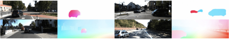
The optical flow is the apparent movement of objects in a scene, concretely we want to know if a car is moving, in which direction or how fast it is moving.
Optical flux provides a concise description of both the regions of the moving image and the speed of movement. In practice, optical flow computation is sensitive to variations in noise and illumination.
It is often used as a good approximation of the actual physical motion projected onto the image plane.

To represent the movement of an object in an image we use movement colors, the color indicates the direction of movement of the object, the intensity the speed of movement.

The traditional approach to deal with an optical flow problem
Optical flow has traditionally been approached as a hand-crafted optimiza- tion problem over the space of dense displacement fields between a pair of images. The concept is to try to determine the velocity of the brightness pattern.
You are going to tell me, how to define the speed of movement of an object in an image with an optimization problem?
The principle is very simple, we define the energy of a pixel or the intensity of a pixel by the following function E(x, y, t) where x and y represents the position of the pixel. The position of the pixel is estimated after a minor change in time to do that it uses derivative. We consider the hypothesis that during a small time variation the intensity of the pixel has not been modified (1).

||uv|| is simply the speed of movement of the pixel within the plane. Traditionally, optical flow problems have been limited to estimating the speed of movement of a pattern within an image. I have introduced the basics of the problem, however we can’t define ||uv||| directly. We have to add other constraints. For those who are interested I leave you the link that explains the method in its entirety link.
RAFT (Recurrent All-Pairs Field Transforms)
RAFT is a new method based on deep learning methods presented at ECCV (European Conference for Computer Vision) 2020 for optical flows. This new method, introduced by Princeton researchers, reduces F1-all error by 16% and becomes the new state of the art for optical flows. RAFT has strong cross-dataset generalization as well as high efficiency in inference time, training speed, and parameter count.
In this article I will present the different bricks that make up RAFT:
- Feature encoder
- multi-scale 4D correlation volumes
- update operator

Feature Encoder
The role of the feature encoder is to extract a vector for each pixel of an image. The feature encoder consists of 6 residual blocks, 2 at 1/2 resolution, 2 at 1/4 resolution, and 2 at 1/8 resolution.
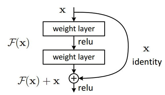
The common culture believes that increasing the depth of a convoluted network increases its accuracy. However, this is a misconception, as increasing the depth can lead to saturation due to problems such as the vanishing gradient. To avoid this, we can add residual blocks that will reintroduce the initial information at the output of the convolution layer and add it up.
Trending AI Articles:
1. Fundamentals of AI, ML and Deep Learning for Product Managers
3. Graph Neural Network for 3D Object Detection in a Point Cloud
4. Know the biggest Notable difference between AI vs. Machine Learning
We additionally use a context network. The context network extracts features only from the first input image 1(Frame 1 on the figure 4). The architecture of the context network, hθ is identical to the feature extraction network. Together, the feature network gθ and the context network hθ form the first stage of this approach, which only need to be performed once.
Multi-Scale 4D correlation volumes
To build the correlation volume, simply apply the dot product between all the output features of the feature encoder, the dot product represents the alignent between all feature vectors. The output is the dimensional correlation volume C(gθ(I1),gθ(I2))∈R^H×W×H×W.
Correlation Pyramid
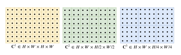
They construct a 4-layer pyramid {C1,C2,C3,C4} by pooling average the last two dimensions of the correlation volume with kernel sizes 1, 2, 4, and 8 and equivalent stride (Figure 6). Only the last two dimensions are selected to maintain high-resolution information that will allow us to better identify the rapid movements of small objects.
C1 shows the pixel-wise correlation, C2 shows the 2×2-pixel-wise correlation, C3 shows the 4×4-pixel-wise.
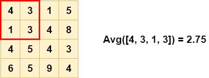
An exemple of average pooling with kernel size = 2, stride = 2. As you can see on figure 7 and 8, Average Pooling compute the average selected by the kernel.
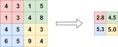
Thus, volume Ck has dimensions H × W × H/2^k× W/2^k . The set of volumes gives information about both large and small displacements.
Correlation Lookup
They define a lookup operator LC which generates a feature map by indexing from the correlation pyramid.
How does indexing work?
Each layer of the pyramid has one dimension C_k = H × W × H/(2^k)× W/(2^k). To index it, we use a bilinear interpolation which consists in projecting the matrix C_k in a space of dimension H × W × H × W.
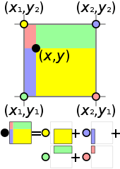
To define a point à coordinate (x, y), we used four points (x1, y2), (x1, y1), (x2, y2) and (x2, y1). Then compute new point (x, y2), (x1, y), (x, y1) and (x2, y) by interpolation, then repeat this step to define (x, y).
Given a current estimate of optical flow (f1,f2), we map each pixel x = (u,v) in image 1 to its estimated correspondence in image 2: x′ = (u + f1(u), v + f2(v)).
Iterative Updates
For each pixel of image 1 the optical flux is initialized to 0, from image 1 we will look for the function f which allows to determine the position of the pixel within image 2 from the multi scale correlation. To estimate the function f, we will simply look for the place of the pixel in image 2.
We will try to evaluate function f sequentially {f1, …, fn}, as we could do with an optimization problem. The update operator takes flow, correlation, and a latent hidden state as input, and outputs the update ∆f and an updated hidden state.
By default the flow f is set to 0, we use the features created by the 4D correlation, and the image to predict the flow. The correlation allows to index to estimate the displacement of a pixel. We then use the indexing between the correlation matrix and image 1 in output of the encoder context to estimate a pixel displacement between image 1 and 2. To do this, a GRU (Gated Recurrent Unit) recurrent network is used. As input the GRU will have the concatenation of the 4D correlation matrix, the flow and image 1 as output of the context encoder. A normal GRU works with fully connected neural networks, but in this case, in order to adapt it to a computer vision problem, it has been replaced by convoluted neural networks.
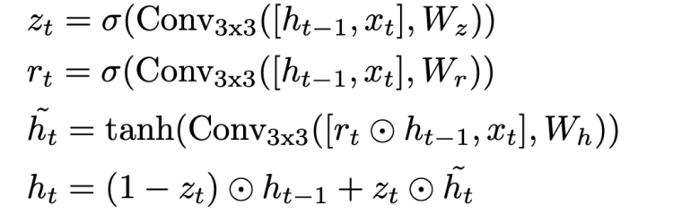
To simplify a GRU works with two main parts : the reset gate that allows to remove non-essential information from ht-1 and the update gate that will define ht. The gate remainder is mainly used to reduce the influence of ht-1 in the prediction of ht. In the case where Rt is close to 1 we find the classical behavior of a recurrent neural network. . This determines the extent to which the new state ht is just the old state ht-1 and by how much the new candidate state ~ht is used.

In our case we use the GRU, to update the optical flow. We use the correlation matrix and image 1 as input and we try to determine the optical flux, i.e. the displacement of a pixel u(x, y) in image 2. We use 10 iteration, i.e. we calculate f10 to estimate the displacement of this pixel.
Loss
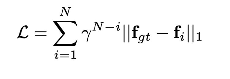
The loss function is defined as the L1 standard between the ground truth flow and the calculated optical flow. We add a Gamma weight that increases exponentially, meaning that the longer the iteration in the GRU the more the error will be penalized. For example let’s take the case where fgt = 2, f0 = 1.5 and f10= 1.8. If we calculate the error L0 = 0.8¹⁰*0.5 = 0.053, L10 = 0.8⁰*0.2=0.2. We quickly understand that an error will be more important at the final iteration than at the beginning.

References
- RAFT (Recurrent All-Pairs Field Transforms for Optical Flow): https://arxiv.org/pdf/2003.12039.pdf
- Determining Optical Flow : http://image.diku.dk/imagecanon/material/HornSchunckOptical_Flow.pdf
- Empirical Evaluation of Gated Recurrent Neural Networks on Sequence Modeling : https://arxiv.org/pdf/1412.3555.pdf
Don’t forget to give us your ? !


Recurrent All-Pairs Field Transforms for Optical Flow was originally published in Becoming Human: Artificial Intelligence Magazine on Medium, where people are continuing the conversation by highlighting and responding to this story.
