
How to evaluate the Machine Learning models? — Part 2
This is second part of the metric series where, we will discuss about correlations — continuous to continuous and dichotomous (categorical) to continuous. When it comes to feature selection in machine learning as well as in dimensionality reduction correlation plays a very crucial role — decides which feature will have high impact on the model and in several cases it is treated as the metric for model evaluation.
Over of correlation matrices if given below, few of them we will be discuss in this article. In first part of this metric series, we have discussed eight statistical metrics, in this part we are going to discuss Correlation Metrics used to evaluate the model as well as feature .
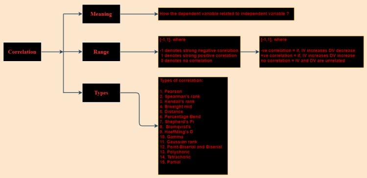
Correlation
Correlation is defined as the relationship between two variable generally IV and DV, it ranges between [-1 ,1], where as -1 means highly negative correlation i.e. increase in D.V will tends to decrease in I.V or vice versa, 0 means no correlation i.e. no relationship exits between I.V and D.V and 1 means highly positive correlation i.e. increase in D.V will tends to increase in I.V or vice versa.
While implementation we use to set threshold for both side, so that we can incorporate the IV which are highly correlated in term of absolute value of magnitude and then we process further to build the model. Below are the correlation metrices:
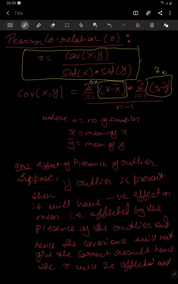
1. Pearson Correlation
Pearson correlation also known as the Pearson’s, the Pearson product- moment correlation coefficient between two variable which is denoted by “r”. It measures linear association between two variable. It is parametric correlation. It ranges from [-1,1] where,
0= no relation,
1= positive relation,
-1 = Negative relation
Pearson Correlation is defined as the covariance of two variable normalized by the product of the standard deviation of the variables.
Assumptions of Pearson Correlation:
- I.V and DV are normally distributed i.e. mean =0 and variance=1 or bell shape curve.
- Both IV and DV are Continuous and as well Linearly related.
- No outliers are present in the IV and as well as DV.
- IV and DV are Homoscedasticity (having the same scatter from the fitted line)

Steps of Pearson Correlation:
- Find the of covariance of X and Y.
2. Find the standard deviation of X and Y.
3. Multiply the covariance of X and Y and divide by multiplication of the standard deviation of X and Y.
Below is the question solved by the Pearson Correlation.

2. Spearman Correlation
Spearman Correlation is a non-parametric test which is used to measure the association between the two variable. It is equal to the Pearson Correlation and it calculated as same as the Pearson Correlation but instead of the value we use rank of the variable. It ranges from [-1,1] where,
0= no relation,
1= positive relation,
-1 = Negative relation
Assumption:
- IV and DV are linear and as well as monotonous.
- IV and DV are Continuous and as well as Ordinal.
- IV and DV are Normally Distributed.
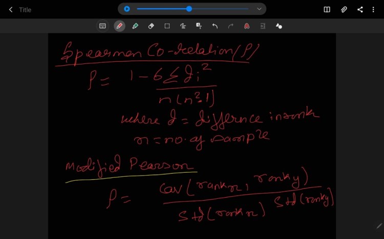
Steps of Spearman Correlation:
- Rank the variable X and Y
- Calculate the difference of the rank i.e. d=R(x)-R(y)
- Raise d to power of 2 and perform summation.
- Calculate n*(n-1), where n is no of the variable.
- Substitute the respective value in the below formulae.
- (optional) you can use the rank of the variable in pearson’s formulae and calculate the Spearman Correlation.

3. Kendall’s Rank Correlation
It is non-parametric measure of the relationship between the columns of the ranked data. It is preferred over Spearman correlation because of the low GES (Gross Error Sensivity) and as well as the Asymptotic Variance. It ranges from [-1,1] where,
0= no relation,
1= positive relation,
-1 = Negative relation
Assumption:
- IV and DV are linear and as well as monotonous.
- IV and DV are Continuous and as well as Ordinal.
- IV and DV are Normally Distributed.
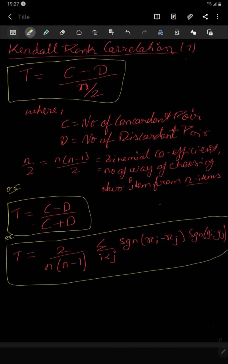
A quirk test can produce the negative coefficient hence making the range between[-1,1] but when we are using ranked data the negative value does no0t mean much. Several version of tau correlation exists such as tau A, Tau B and Tau C. Tau a used with squared table (no. of row==no. of columns), and Tau C for rectangular columns.
Trending AI Articles:
1. Fundamentals of AI, ML and Deep Learning for Product Managers
3. Graph Neural Network for 3D Object Detection in a Point Cloud
4. Know the biggest Notable difference between AI vs. Machine Learning
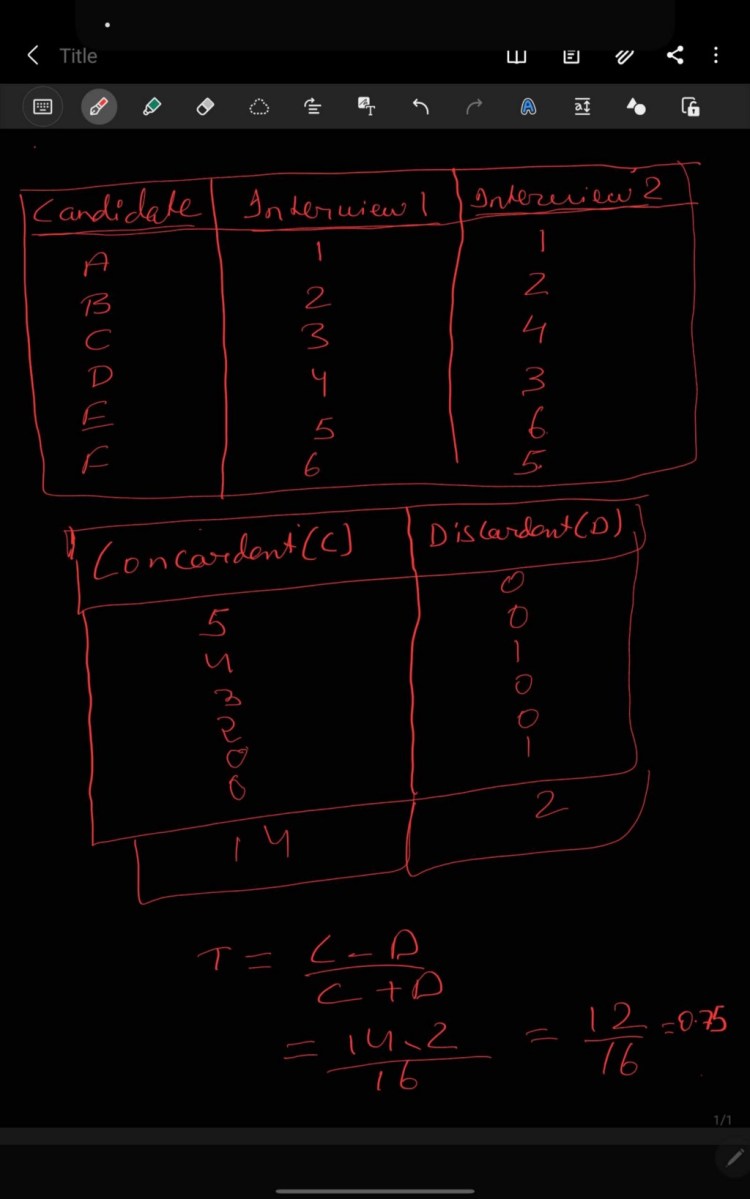
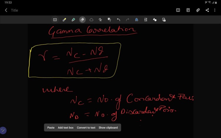
Kendal tau= (C-D)/(C+D) where,
C is concordant and D is Discordant.
Briefly, Concordant means rank are ordered in same order irrespective of the rank(X increases Y also increases)and Discordant (X increases Y also decreases )means rank are ordered in opposite way irrespective of rank.
Steps of Kendall’s Rank Correlation:
Steps to find Concordant:
- Take any column, in below image, i have taken Interviewer 2.
- For first value in the selected feature i.e. Interviewer 2, count no of value in the respective column starting from next row which is greater than the selected value in row . Suppose you are calculating concordant for ith row, so you will take values from (i+1)th row from the Interview column.
Steps to find Discordant:
- Take any column, in below image, i have taken Interviewer 2.
- For first value in the selected feature i.e. Interviewer 2, count no of value in the respective column starting from next row which is smaller than the selected value in row . Suppose you are calculating concordant for ith row, so you will take values from (i+1)th row from the Interview column.
4. Distance Correlation
Distance correlation is used to test the relation between the IV and DV which are Linear or Nonlinear, in contrast with the Pearson which is applicable to only Linear related data. Statistical test of dependence can be performed with a permutation test. It ranges from 0,1 where,
0= no relation,
1= positive relation,
-1 = Negative relation
Steps of Distance Correlation:
- Calculate distance metric of X and Y .
- Calculate doubly center for X and Y each element.
- Multiply the doubly center of X and Y for each term take the summation and finally divide by n raised to 2.

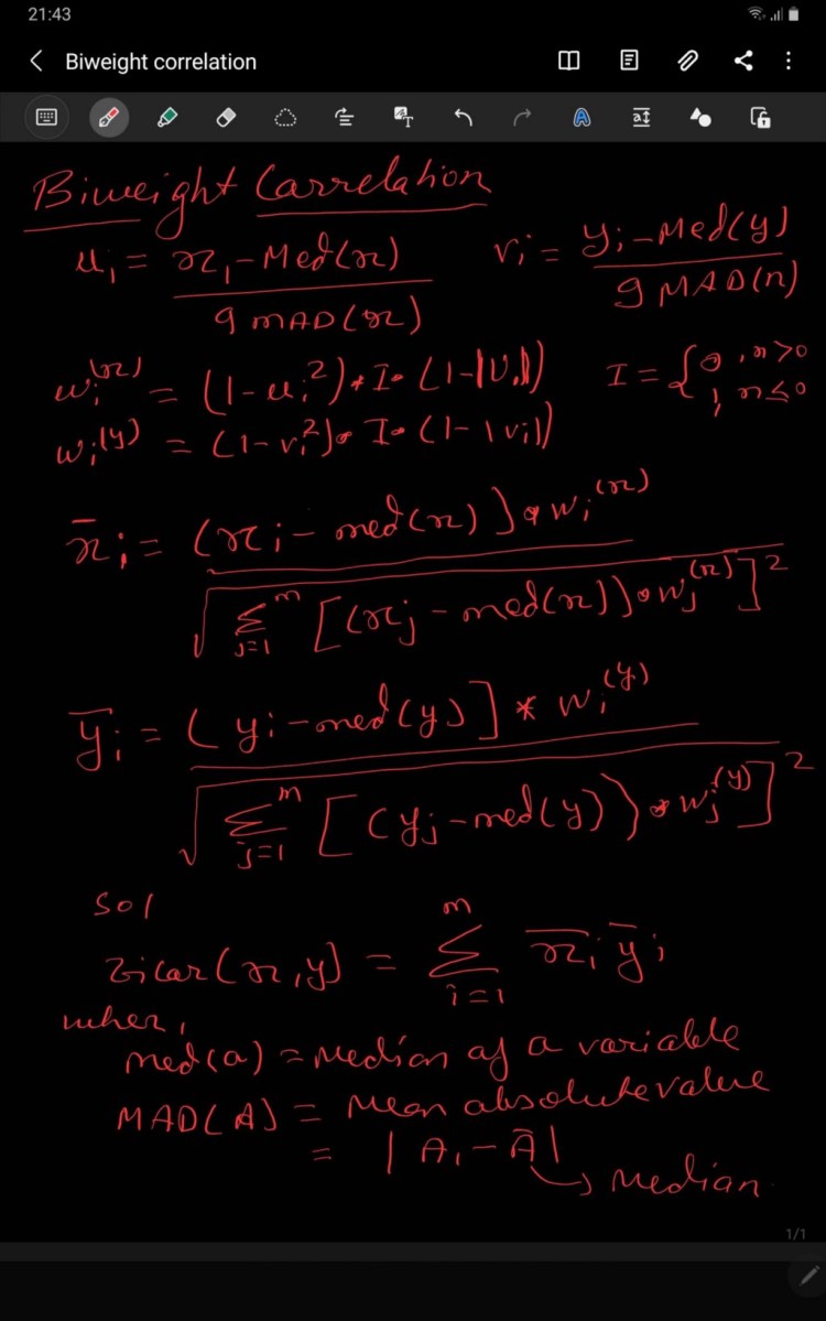
5. Biweight MidCorrelation
This type of correlation is median base instead of traditionally mean base, also know as bicorr – measures similarity between samples. It is less affected by outlier because it is independent of mean. It ranges from 0,1 where,
0= no relation,
1= perfect relation.
1= negative perfect relation.
Assumptions of Biweight MidCorrelation:
- I.V and DV are normally distributed i.e. mean =0 and variance=1 or bell shape curve.
- Both IV and DV are Continuous or ordinal.
Steps of Distance Correlation:
Follow the instruction/steps mentioned in the below image:
6. Gamma Correlation
It is measurement of rank correlation equivalent to the Kendal rank correlation. It is robust to outliers. It’s goal is to predict where new value will rank. It is applicable to data which are tied with their respective rank. It ranges from 0,1 where,
0= no relation,
1= perfect relation.
1= negative perfect relation.
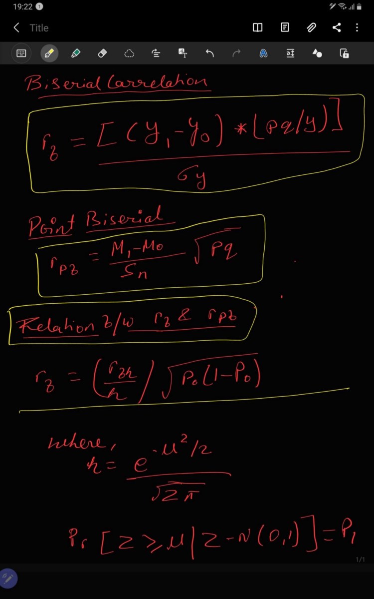
7. Point Biserial Correlation
This type of of the correlation is used to calculate the relationship between dichotomous(binary) variable and continuous variable works well then IV and DV are linearly dependent. IT is same as the Pearson correlation the only difference is that it works with dichotomous and continuous variable. It ranges from 0,1 where,
0= no relation,
1= perfect relation.
1= negative perfect relation.
Assumptions of Point Biserial Correlation:
- I.V and DV are normally distributed i.e. mean =0 and variance=1 or bell shape curve.
- Anyone of them IV or DV should Continuous or ordinal and another should be dichotomous.
Formulae and Steps of Point Biserial Correlation:
Follow the instruction/steps mentioned in the below image:

8. Biserial correlation
Biserial correlation is almost the same as point biserial correlation, but one of the variables is dichotomous ordinal data and has an underlying continuity. It ranges from 0,1 where,
0= no relation,
1= perfect relation.
1= negative perfect relation.
Assumptions of Biserial correlation :
- I.V and DV are normally distributed i.e. mean =0 and variance=1 or bell shape curve.
- Anyone of them IV or DV should ordinal which has underlying continuity and another should be dichotomous.
Steps of Biserial correlation:
Follow the instruction/steps mentioned in the below image:
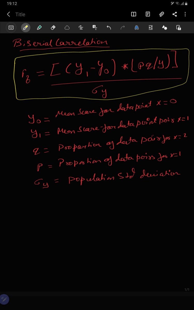
Relationship between Biserial correlation and Point Biserial Correlation.
9. Partial Correlation
Partial correlation we measure the strength of correlation between the variable by controlling one or more variable. Like if dataset has 5 IV then we calculate correlation with 1 IV and DV and then we calculate correlation between 2 IV and DV and so on. Therefore some discrepancies is there when we compare t and p-value from other correlation method.
Special Thanks:
As we say “Car is useless if it doesn’t have a good engine” similarly student is useless without proper guidance and motivation. I will like to thank my Guru as well as my Idol “Dr. P. Supraja”- guided me throughout the journey, from bottom of my heart. As a Guru, she has lighted the best available path for me, motivated me whenever I encountered failure or roadblock- without her support and motivation this was an impossible task for me.
Contact me:
If you have any query feel free to contact me on any of the below-mentioned options:
Website: www.rstiwari.com
Google Form: https://forms.gle/mhDYQKQJKtAKP78V7
Notebook for Reference:
Jovian Notebook: https://jovian.ai/tiwari12-rst/correlation
Jovian Notebook: https://jovian.ml/tiwari12-rst/metrices-part1
References:
Correlation Types: https://easystats.github.io/correlation/articles/types.html
Environment Set-up: https://medium.com/@tiwari11.rst
Youtube : https://www.youtube.com/channel/UCFG5x-VHtutn3zQzWBkXyFQ
Don’t forget to give us your ? !


How to evaluate the Machine Learning models? — Part 2 was originally published in Becoming Human: Artificial Intelligence Magazine on Medium, where people are continuing the conversation by highlighting and responding to this story.
