
ML05: Neural Network on iris by Numpy
Discover NN elements by a perceptron from scratch
Read time: 10~12 min
Beginners of NN often intimidated by the tricky math and complex models at the first sight, so I'd like to share a fairly simple toy example of NN on iris without leveraging any DL framework like PyTorch or Tensorflow from a book written by Japanese[1], and only by NumPy----that is, we need to create the loss functions, activators, and adjusting weights on our own.
Complete Python code:
https://drive.google.com/drive/folders/1Haknut4yGujlWP-QKpJnFWwRJE1xtf9Y
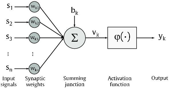
Neuron is a minimum unit of neural network. A perceptron is a single-layer neural network. Let’s try to do a binary classification of iris by a perceptron.
Outline
(1) Dataset
(2) Neural Network Review
(3) Input
(4) Data Splitting
(5) Define Functions
(6) Training
(7) Testing
(8) Summary
(9) Reference

(1) Dataset
The renowned iris from:
https://archive.ics.uci.edu/ml/machine-learning-databases/iris/iris.data
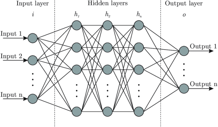
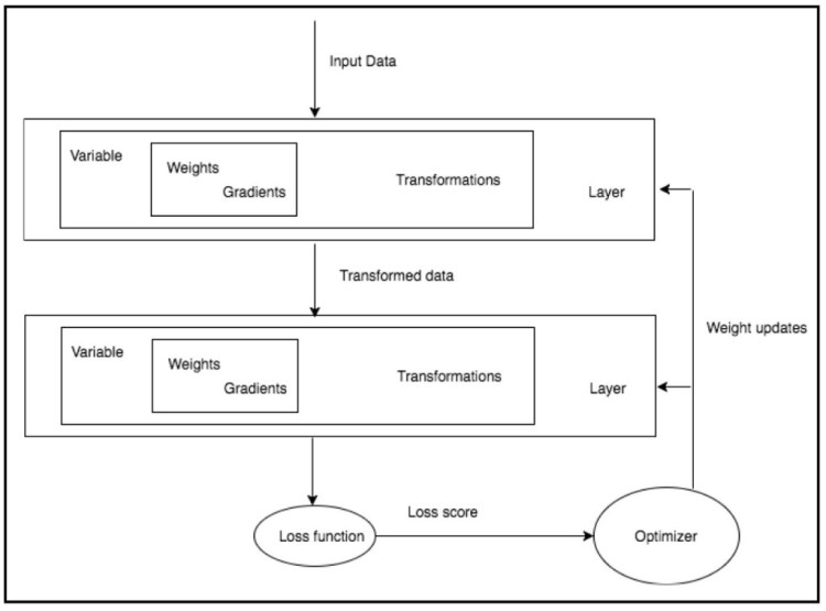
(2) Neural Network Review
(3) Input
import numpy as np
import pandas as pd
import os
os.chdir("D:\\Python\\Numpy_JP\\ch04-3")
# Choose your own working directory
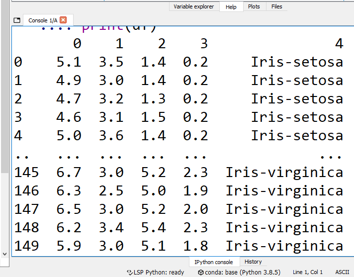
df = pd.read_csv('iris.data', header=None)
print(df)
Trending AI Articles:
We would have the following data frame of iris:
x = df.iloc[0:100,[0, 1, 2, 3]].values
y = df.iloc[0:100,4].values
y = np.where(y=='Iris-setosa', 0, 1)
We take the first 100 rows, and divide the dataset into x (feature) & y (target). Then np.where transform the nominal data y from text to numeric.
(4) Data Splitting
x_train = np.empty((80, 4))
x_test = np.empty((20, 4))
y_train = np.empty(80)
y_test = np.empty(20)
x_train[:40],x_train[40:] = x[:40],x[50:90]
x_test[:10],x_test[10:] = x[40:50],x[90:100]
y_train[:40],y_train[40:] = y[:40],y[50:90]
y_test[:10],y_test[10:] = y[40:50],y[90:100]
Row 1~50 are “Iris-setosa”, and row 51~100 are “Iris-virginica.” So we collect row 1~40 of and row 51~90 to be the training set, and the rest rows are testing set.
(5) Define Functions
def sigmoid(x):
    return 1/(1+np.exp(-x))
def activation(x, w, b):
    return sigmoid(np.dot(x, w)+b)
def update(x, y_train, w, b, eta):
    y_pred = activation(x, w, b)
    # activator
    a = (y_pred - y_train) * y_pred * (1- y_pred)
    # partial derivative loss function
    for i in range(4):
        w[i] -= eta * 1/float(len(y)) * np.sum(a*x[:,i])
    b -= eta * 1/float(len(y))*np.sum(a)
    return w, b
Let’s probe into the math behind the preceding code:

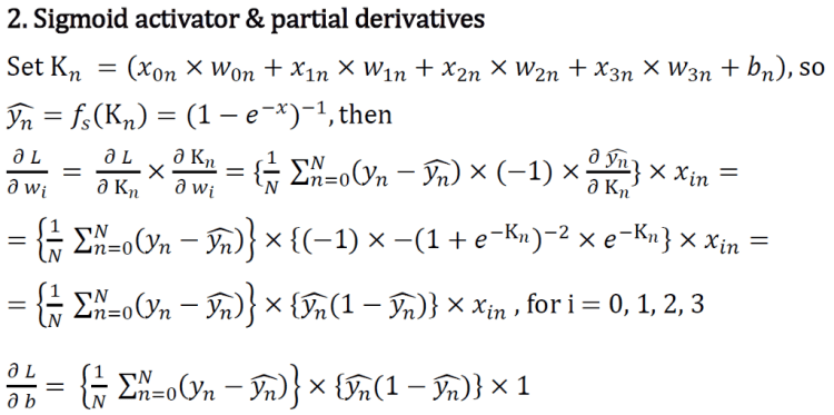


- Activator: sigmoid function
- Loss function: MSE (mean square error)
- Optimizer: gradient descend
- Weight updates: tiresome math work
(6) Training
weights = np.ones(4)/10
bias = np.ones(1)/10
eta = 0.1
for _ in range(15): # Run both epoch=15 & epoch=100
 weights, bias = update(x_train, y_train, weights, bias, eta=0.1)
- Initial weights: Let wi & b all be 0.1
- Learning rate: set eta= 1
- Epoch: Run both epoch= 15 & epoch= 100
(7) Testing
print("Epochs = 15") # Run both epoch=15 & epoch=100
print('weights = ', weights, 'bias = ', bias)
print("y_test = {}".format(y_test))
activation(x_test, weights, bias)
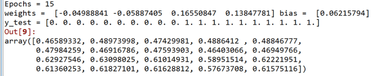

If we set the decision boundary at 0.5, then we get 100% accuracy in both epochs = 15 & 100.
The first 10 predictions of epochs = 15 are between 0.46~0.49, while the first 10 predictions of epochs = 100 are between 0.23~0.30. The last 10 predictions of epochs = 15 are between 0.57~0.63, while the last 10 predictions of epochs = 100 are between 0.64~0.81. As epochs rises, values of the two flower group become more distance.
(8) Summary
Without any NN framework, we built up a single-layer neural network ! We discovered concepts like activator(sigmoid), loss function(MSE), optimizer(gradient descend), weight updates(tiresome math work), initial weights(wi = b= 1), learning rate(eta= 1), epoch(tried epochs= 15 & 100).
(9) Reference
[1] Yoshida, T. & Ohata, S. (2018). Genba de Tsukaera! NumPy Data Shori Nyumon kikaigakushu| datascience de yakudatsu kosoku shorishuho. Japan, JP: SHOEISHA.
[2] Bre, F. et al(2020). An efficient metamodel-based method to carry out multi-objective building performance optimizations. Energy and Buildings, 206, (unknown).
[3] Subramanian, V. (2018). Deep Learning with PyTorch. Birmingham, UK: Packt Publishing.
[4] Roughgarden, T. & Valiant, G.(2015). CS168: The Modern Algorithmic Toolbox Lecture #15: Gradient Descent Basics. Retrieved from
http://theory.stanford.edu/~tim/s15/l/l15.pdf
Don’t forget to give us your ? !


ML05: Neural network on Iris was originally published in Becoming Human: Artificial Intelligence Magazine on Medium, where people are continuing the conversation by highlighting and responding to this story.
Via https://becominghuman.ai/ml05-8771620a2023?source=rss—-5e5bef33608a—4
source https://365datascience.weebly.com/the-best-data-science-blog-2020/ml05-neural-network-on-iris
