
Here , we have implemented a knowledge graph from a WikiPedia actors dataset. The article [1] by analyticsvidya has been heavily referred for this. But we have made improvements in the form of :
- Data Preprocessing — Removed punctuations , stop words
- Named Entity Recognition — This has helped in constructing a more meaningful graph with less noise.
Using Named Entity Recognition has helped us obtain top occuring Actors, writers,stuidio names etc
import re
import pandas as pd
import spacy
from tqdm import tqdm
# Load English tokenizer, tagger, parser, NER and word vectors
nlp = spacy.load("en_core_web_sm")
from spacy.matcher import Matcher
import networkx as nx
import matplotlib.pyplot as plt
import nltk
from nltk.tokenize import word_tokenize
from nltk.corpus import stopwords
import re
import string
tqdm._instances.clear()
from google.colab import drive
drive.mount('/content/drive')
Mounted at /content/drive

Importing data from csv and storing in a pandas dataframe
data_dir = "/content/drive/My Drive/data/wiki_sentences_v2.csv"
sentences = pd.read_csv(data_dir)
sentences.shape
(4318, 1)
sentences.head()
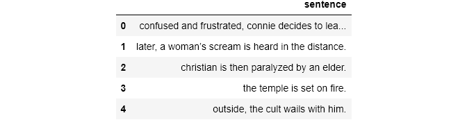
Here are some sample sentences containing the words “bollywood” and “contemporary” together
Trending AI Articles:
sentences[sentences['sentence'].str.contains('bollywood' and 'contemporary')]

Entity Pairs Extraction Function
def get_entity(sent):
  ent1 = "" #subject entity
  ent2 = "" #object entity

  prev_token_text = "" #text from previous token
  prev_token_dep = ""  #depedency from previous token

  prefix = ""
  modifier = ""

  for tok in nlp(sent):
    #Go in only if it is not a punctuation, else next word
    if tok.dep_ != "punct":
      #Check if token is a compund word
      if tok.dep_ == "compound":
        prefix = tok.text
        #Check if previous token is also a compound
        if prev_token_dep == "compound":
          prefix = prev_token_text + " "+ prefix
      #Check if token is a modifier or not
      if tok.dep_.endswith("mod")==True:
        modifier = tok.text
        #Check if previous token is a compound
        if prev_token_dep == "compound":
          modifier = prev_token_text + " " + modifier

      #Checking if subject
      if tok.dep_.find("subj") == True:
        ent1 =modifier+ " " + prefix + " " + tok.text
        prefix = ""
        modifer = ""
      #Checking if object
      if tok.dep_.find("obj") == True:
        ent2 =modifier+ " " + prefix + " " + tok.text
        prefix = ""
        modifer = ""

      #Update variables
      prev_token_text = tok.text
      prev_token_dep = tok.dep_

      ############################
  return [ent1.strip(), ent2.strip()]
Now lets obtain entity pairs from a sentence
[ent1,ent2] = get_entity("the film had 200 patents")
print("Subj : {a}, obj : {b}".format(a = ent1, b = ent2))
get_entity("the film had 200 patents")
Subj : film, obj : 200  patents


['film', '200  patents']
entity_pairs = []
for i in tqdm(sentences['sentence']):
  entity_pairs.append(get_entity(i))
tqdm._instances.clear()
100%|██████████| 4318/4318 [00:41<00:00, 103.43it/s]
subjects = []
objects = []
subjects = [x[0] for x in entity_pairs]
objects = [x[1] for x in entity_pairs]
Relation Extraction
The Relation between nodes has been extracted. The hypothesis is that the main verb or the Root word forms the relation between the subject and the object.
def get_relation(sent):
  doc = nlp(sent)
  #We initialise matcher with the vocab
  matcher = Matcher(nlp.vocab)
  #Defining the pattern
  pattern = [{'DEP':'ROOT'},{'DEP':'prep','OP':'?'},{'DEP':'agent','OP':'?'},{'DEP':'ADJ','OP':'?'}]
  #Adding the pattern to the matcher
  matcher.add("matcher_1",None,pattern)
  #Applying the matcher to the doc
  matches = matcher(doc)

  #The matcher returns a list of (match_id, start, end). The start to end in our doc contains the relation. We capture that relation in a variable called span
  span = doc[matches[0][1]:matches[0][2]]
  return span.text
Below we observe a problem. The Relation for the second should be “couldn’t complete”, in order to correctly capture the semantics. But it fails to do so.
get_entity("John completed the task"), get_relation("John completed the task")
(['John', 'task'], 'completed')
get_entity("John couldn't complete the task"), get_relation("John couldn't complete the task")
(['John', 'task'], 'complete')
Anyway, we move on. Let’s get the relations for the entire dataset
relations = [get_relation(i) for i in tqdm(sentences['sentence'])]
tqdm._instances.clear()
100%|██████████| 4318/4318 [00:41<00:00, 102.82it/s]
Let’s look at the topmost occuring subjects
pd.Series(subjects).value_counts()[:10]
it       267
film     222
         147
he       141
they      66
i         64
this      55
she       41
we        27
films     25
dtype: int64
We observe that these words are mostly generic, hence of not much use to us.
pd.Series(relations).value_counts()[:10]
is          418
was         340
released    165
are          98
were         97
include      81
produced     51
's           50
made         46
used         43
dtype: int64
Not surprisingly, “is” and “was” forms the most common relations, simply because they are the most common words. We want more meaningful subjects to be more prominent.
Data Pre — Processing
Let’s see what happens if we pre-process the data. We remove stopwords and punctuation marks
def isNotStopWord(word):
    return word not in stopwords.words('english')

def preprocess(sent):
  sent = re.sub("[\(\[].*?[\)\]]", "", sent)
  tokens = []
  temp = ""
  words = word_tokenize(sent)
  # Removing punctuations except '<.>/<?>/<!>'
  punctuations = '"#$%&\'()*+,-/:;<=>@\\^_`{|}~'
  words = map(lambda x: x.translate(str.maketrans('','',punctuations)), words)

  #Now, we remove the stopwords
  words = map(str.lower,words)
  words = filter(lambda x: isNotStopWord(x),words)
  tokens = tokens + list(words)
  temp = ' '.join(word for word in tokens)
  return temp
preprocessed_sentences = [preprocess(i) for i in tqdm(sentences['sentence'])]
tqdm._instances.clear()
100%|██████████| 4318/4318 [00:06<00:00, 659.03it/s]
Getting entity pairs from preprocessed sentences
entity_pairs = []
for i in tqdm(preprocessed_sentences):
  entity_pairs.append(get_entity(i))
tqdm._instances.clear()
100%|██████████| 4318/4318 [00:38<00:00, 111.16it/s]
relations = [get_relation(i) for i in tqdm(preprocessed_sentences)]
tqdm._instances.clear()
100%|██████████| 4318/4318 [00:39<00:00, 109.65it/s]
pd.Series(relations).value_counts()[:10]
released    173
include      81
produced     62
directed     52
made         50
film         48
used         42
became       35
began        35
included     34
dtype: int64
We see above that only the important relations are present, “released” being the most common. There is no “is”, “was” and trivial words as before.This fulfils our desire if eliminating noise.
What if we only want Named Entities to be present? Entities like Actors, Films, Studios, Composers etc
entity_pairs2 = entity_pairs
relations2 = relations
#We keep relations only for those entities whose both source and target are present
entity_pairs3 = []
relations3 = []
for i in tqdm(range(len(entity_pairs2))):
  if entity_pairs2[i][0]!='' and entity_pairs2[i][1]!='':
    entity_pairs3.append(entity_pairs2[i])
    relations3.append(relations2[i])
tqdm._instances.clear()
100%|██████████| 2851/2851 [00:00<00:00, 482837.79it/s]
As we observe, the number of relations decrease to 2851 . Previously it was around 4k
Named Entity Recognition Using Spacy
source = []
target = []
edge = []
for i in (range(len(entity_pairs))):
  doc_source = nlp(entity_pairs[i][0]).ents #Getting the named entities for source
  #Converting the named entity tuple to String
  str_source = [str(word) for word in doc_source]
  doc_source = ' '.join(str_source)
  doc_target = nlp(entity_pairs[i][1]).ents #Getting the named entities for target
  #Converting the named entity tuple to String
  str_target = [str(word) for word in doc_target]
  doc_target = ' '.join(str_target)
  if doc_source != '' or doc_target != '':
    edge.append(relations[i])
    source.append(entity_pairs[i][0])
    target.append(entity_pairs[i][1])
We had obtained entity pairs before but they had many irrelevant words. We narrowed them down quite a bit by preprocessing. Now, we obtain the named entity pairs which will form source and target respectively. It looks like (source, target, edge). We prune this further by removing all the data which have neither source or target entity as a Named Entity. We keep the rest. The Relations that were extracted before form the edge
Now, we find the most popular Source , Target and Relations
print("###################  Most popular source entites    ###################### \n",pd.Series(source).value_counts()[:10])
print("###################  Most popular target entites    ###################### \n",pd.Series(target).value_counts()[:10])
print("###################  Most popular relations         ###################### \n",pd.Series(relations).value_counts()[:20])
###################  Most popular source entites    ######################
                           165
film                       64
khan                       10
first  film                 9
movie                       6
indian  film                6
two certificate awards      5
music                       5
series                      5
films                       4
dtype: int64
###################  Most popular target entites    ######################
                                242
warner bros                      7
national film awards             5
film                             4
positive box office success      4
surviving studio india           4
1980s                            3
british film institute           3
undisclosed  roles               3
positive  reviews                3
dtype: int64
###################  Most popular relations         ######################
 released      173
include        81
produced       62
directed       52
made           50
film           48
used           42
became         35
began          35
included       34
films          32
composed       31
become         30
written        27
shot           27
set            26
received       26
introduced     25
considered     22
called         22
dtype: int64
Constructing the Knowledge Graph
We first take the knowledge graph in a pandas dataframe. It will be a directional graph.
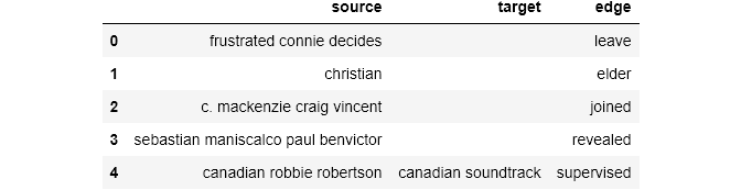
knowledge_graph_df = pd.DataFrame({'source':source, 'target':target, 'edge':edge})
knowledge_graph_df.head()
#MultiDIGRaph because its a directional graph
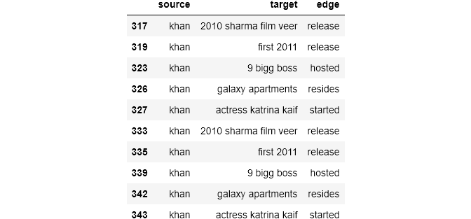
Let’s see what we get when the source enity is “khan”
knowledge_graph_df[knowledge_graph_df['source']=="khan"]
G = nx.from_pandas_edgelist(knowledge_graph_df[knowledge_graph_df['source']=="khan"],source = 'source', target = 'target', edge_attr = True, create_using= nx.MultiDiGraph())
#MultiDIGRaph because its a directional graph
plt.figure(figsize = (10,10))
pox = nx.spring_layout(G,k = 1.0) #k defines the distnace between nodes
nx.draw(G, with_labels= True, node_size = 2500)
plt.show()
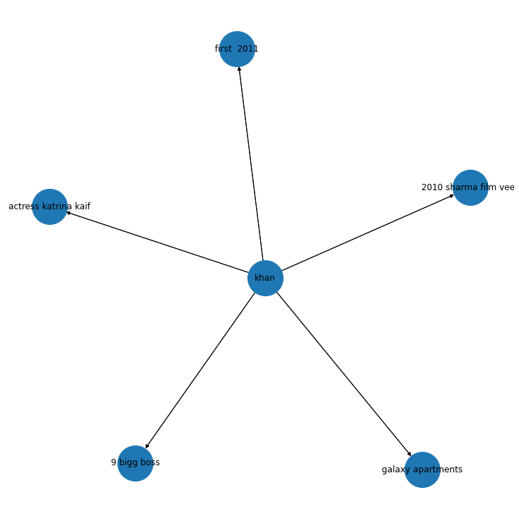
We observe that “khan” points to “actress katrina kaif” , “big boss” and “2010 film Veer”.
Pretty obvious which “khan” is indicated here.


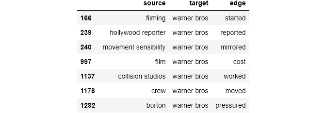
This is what we get when the target is “Warner bros”
knowledge_graph_df[knowledge_graph_df['target']=="warner bros"]
G = nx.from_pandas_edgelist(knowledge_graph_df[knowledge_graph_df['target']=="warner bros"],source = 'source', target = 'target', edge_attr = True, create_using= nx.MultiDiGraph())
plt.figure(figsize = (10,10))
pox = nx.spring_layout(G,k = 1.0) #k defines the distnace between nodes
nx.draw(G, with_labels= True, node_size = 2500)
plt.show()
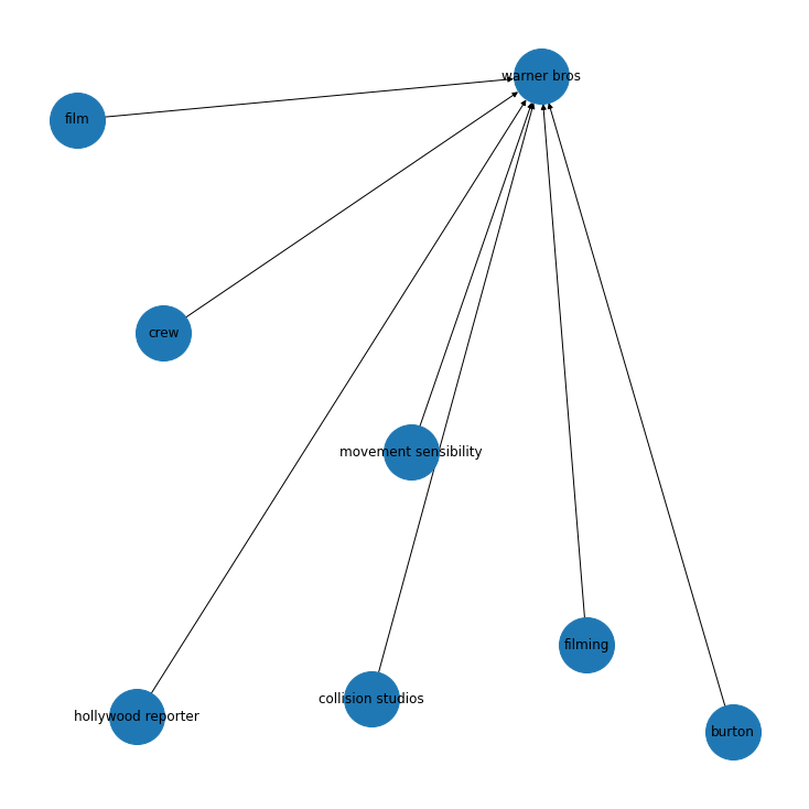
So, for a very small dataset, we get some interesting graph structures which match with our intuition. We can further develop on this by taking a larger dataset and calculating some measures ,like degree centrality etc.
References
Don’t forget to give us your ? !


Building a small knowledge graph using NER was originally published in Becoming Human: Artificial Intelligence Magazine on Medium, where people are continuing the conversation by highlighting and responding to this story.
