365 Data Science is an online educational career website that offers the incredible opportunity to find your way into the data science world no matter your previous knowledge and experience.
Data that is updated in real-time requires additional handling and special care to prepare it for machine learning models. The important Python library, Pandas, can be used for most of this work, and this tutorial guides you through this process for analyzing time-series data.
Also: Online Certificates/Courses in #AI, #BusinessAnalytics, #DataScience, #MachineLearning from Top Universities; 24 Best (and #Free) #Books To Understand #MachineLearning; New Poll: What Python IDE / Editor you used the most in 2020?; Mathematics for #MachineLearning: The #Free eBook
The first in a series of blogs by FICO’s Benjamin Baer introduces the role of decision management as a critical means to help data-driven insights drive your business decisions.
Academically, it is a well-established area of computer science and many decades worth of research work have gone into this field. However, the use of deep neural networks has recently revolutionized the CV field and given it new oxygen.
Big Data Jobs
There is a diverse array of application areas for computer vision. In this article, we briefly show you the common challenges associated with a CV system when it employs modern ML algorithms. For our discussion, we focus on two of the most prominent (and technically challenging) use cases of computer vision:
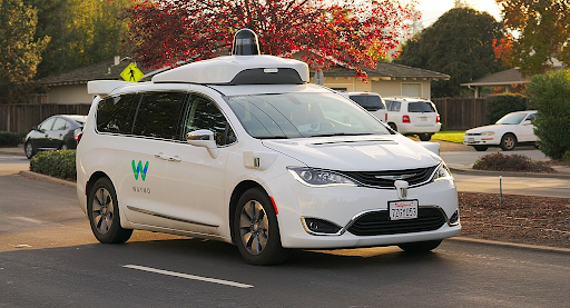
Autonomous driving
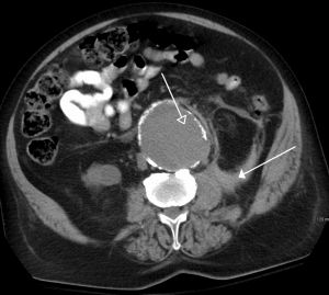
Medical imaging analysis and diagnostics
Both of these use cases present a high degree of complexity, along with other associated challenges.
Challenges Associated with Computer Vision (CV) in Machine Learning (ML)
A common challenge is the large number of tasks associated with a given use case. For example, the autonomous driving use case includes not only object detection but also object classification, segmentation, motion detection, etc. On top of it, these systems are expected to make this kind of CV processing happening in a fraction of a second, and convey a high-probability decision to the higher-level supervisory control system responsible for the ultimate task of driving.
Furthermore, not one, but multiple such CV systems/algorithms are often at play in any respectable autonomous driving system. The demand for parallel processing is high in those situations and this leads to high stress on the underlying computing machinery. If multiple neural networks are used at the same time, they may be sharing the common system storage and compete with each other for a common pool of resources.
In the case of medical imaging, the performance of the computer vision system is judged against highly experienced radiologists and clinical professionals who understand the pathology behind an image. Moreover, in most cases, the task involves identifying rare diseases with very low prevalence rates. This makes the training-data sparse and rarefied (i.e. not enough training images can be found). Consequently, the Deep Learning (DL) architecture has to compensate for this by adding clever processing and architectural complexity. This, of course, leads to enhanced computational complexity.
Learn how Artificial Intelligence (AI) is changing medical imaging into one of the fastest growing deep learning healthcare segments. Download Whitepaper
Popular Datasets for Computer Vision (CV) Tasks
Training machines on image and video files is a serious data-intensive operation.
A singular image file is a multi-dimensional, multi-megabytes digital entity containing only a tiny fraction of ‘insight’ in the context of the whole ‘intelligent image analysis’ task. In contrast, a similar-sized sales data table can lend much more insight into the ML algorithm with the same expenditure on the computational hardware. This fact is worth remembering while talking about the scale of data and the computing required for modern computer vision pipelines.
Unfortunately, one or two (or even a set of hundred) images is usually not enough to fully train on. Robust, generalizable, production-quality deep learning systems require millions of images to train on.
Here, we list some of the most popular ones (consisting of both static images and video clips):
ImageNet
ImageNet is an ongoing research effort to provide researchers around the world with an easily accessible image database. This project is inspired by a growing sentiment within the image and vision research field — the need for more data. It is organized according to the WordNet hierarchy. Each meaningful concept in WordNet, possibly described by multiple words or word phrases, is called a “synonym set” or “synset”. There are more than 100,000 synsets in WordNet. ImageNet aims to provide on average 1000 images to illustrate each synset.
IMDB-Wiki
This is one of the largest and open-sourced datasets of face images with gender and age labels for training. In total, there are 523,051 face images in this dataset where 460,723 face images are obtained from 20,284 celebrities from IMDB and 62,328 from Wikipedia.
MS Coco
COCO or Common Objects in Context is a large-scale object detection, segmentation, and captioning dataset. The dataset contains photos of 91 object types which are easily recognizable and have a total of 2.5 million labeled instances in 328k images.
MPII Human Pose
This dataset is used for the evaluation of articulated human pose estimation. It includes around 25K images containing over 40K people with annotated body joints. Here, each image is extracted from a YouTube video and provided with preceding ann following un-annotated frames. Overall the dataset covers 410 human activities and each image is provided with an activity label.
20BN-SOMETHING-SOMETHING
This dataset is a large collection of densely-labeled video clips that show humans performing pre-defined basic actions with everyday objects. It was created by a large number of crowd workers which allows ML models to develop a fine-grained understanding of basic actions that occur in the physical world.
Storage Requirements for Large-Scale Computer Vision (CV) Tasks
It’s needless to emphasize that to work with such large-scale datasets, many of which are continuously updated and expanded, engineers need robust, fail-proof, high-performance storage solutions to be an integral part of a DL-based CV system. In real-life scenarios, terabytes of image/video data can be generated within a short span of time by end-of-line systems like automobile/drone cameras or x-ray/MRI machines in a network of hundreds of hospitals/clinics.
That seriously puts a whole new spin on the term “Big Data.”
There are multiple considerations and dimensions of choosing and adopting the right data storage for your computer vision task. Some of them are as follows,
Data formats: A wide variety of data formats, including binary large object (BLOB) data, images, video, audio, text, and structured data, which have different formats and I/O characteristics.
Architecture at scale: Scale-out system architecture in which workloads are distributed across many storage nodes/sub-clusters, for training, and potentially hundreds or thousands of nodes for the inference job.
Bandwidth and throughput considerations and optimizations that can rapidly deliver massive quantities of parallel data to compute hardware flowing through these storage nodes.
IOPS, that can sustain high throughput regardless of the data-flow characteristics — that is, for both multitude of small transactions and fewer large transfers.
Latency to deliver data with minimal lag since, as with virtual memory paging, the performance of training algorithms can significantly degrade when GPUs are kept waiting for a new batch of data.
Gaming Chips (GPUs) Are The New Workhorses
General-purpose CPUs struggle when operating on a large amount of data e.g., performing linear algebra operations on matrices with tens or hundreds thousand floating-point numbers. Under the hood, deep neural networks are mostly composed of operations like matrix multiplications and vector additions.
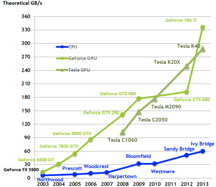
GPUs were developed (primarily catering to the video gaming industry) to handle a massive degree of parallel computations using thousands of tiny computing cores. They also feature large memory bandwidth to deal with the rapid dataflow (processing unit to cache to the slower main memory and back), needed for these computations when the neural network is training through hundreds of epochs. This makes them the ideal commodity hardware to deal with the computation load of computer vision tasks.
This is a nice graphical comparison of GPU vs. CPU from thisMedium post:
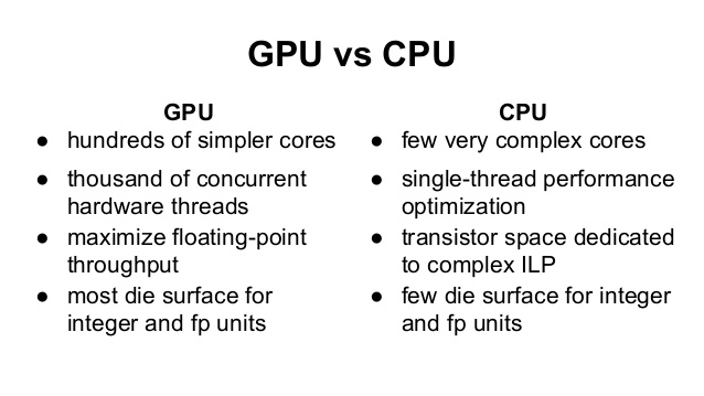
And here is a simple table summarizing the key differences (from this post):
On a high-level, the main features you need to look for while choosing a GPU for your DL system, are:
Memory bandwidth
Raw processing power — for example, the number of CUDA cores multiplied by the clock speed
Amount of the video RAM (i.e. the amount of data you can load on the video/GPU card at once). For time-sensitive CV tasks, this is crucial to be as large as possible because you don’t want to waste valuable clock cycles by fetching the data in small batches from the main memory (the standard DRAM of your system).
Examples of GPU Benchmarking for Computer Vision (CV) Tasks
There are many choices of GPUs on the market, and this can certainly overwhelm the average user with trying to figure out what to buy for their system. There are some good benchmarking strategies that have been published over the years to guide a prospective buyer in this regard.
Also, multiple dimensions of performance must be considered for a good benchmark. For example, the article above mentions three primary indices:
SECOND-BATCH-TIME: Time to finish the second training batch. This number measures the performance before the GPU has run long enough to heat up. Effectively, no thermal throttling.
AVERAGE-BATCH-TIME: Average batch time after 1 epoch in ImageNet or 15 epochs in CIFAR. This measure takes into account thermal throttling.
SIMULTANEOUS-AVERAGE-BATCH-TIME: Average batch time after 1 epoch in ImageNet or 15 epochs in CIFAR with all GPUs running simultaneously. This measures the effect of thermal throttling in the system due to the combined heat given off by all GPUs.
An older but highly popular and rigorously tested benchmarking exercise can be found in this open-source Github repo (there have been many GPU advances since then, with a new line from NVIDIA that blow away older GPUs in performance: RTX 3070, RTX 3080, RTX 3090).
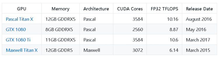
The table from this exercise looks like the following:
Benchmarked GPUs
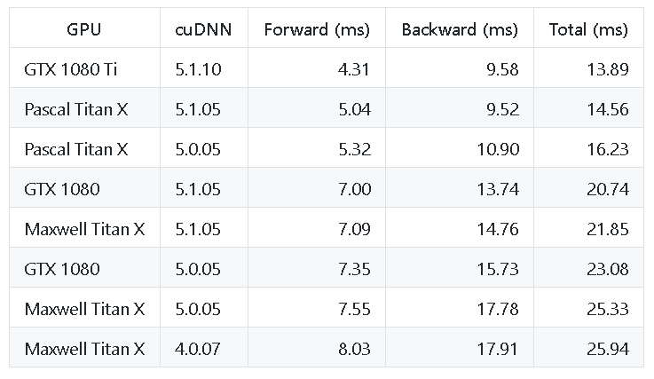
AlexNet Performance
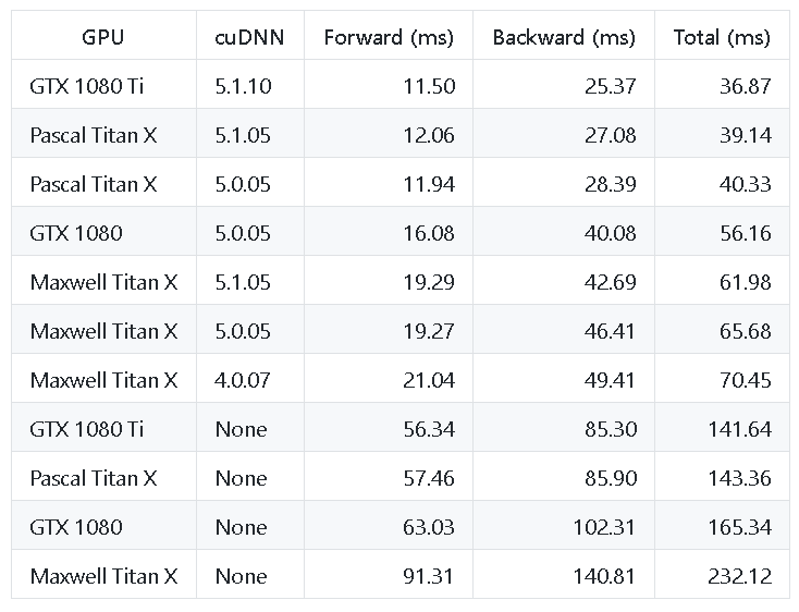
Inception V1 Performance
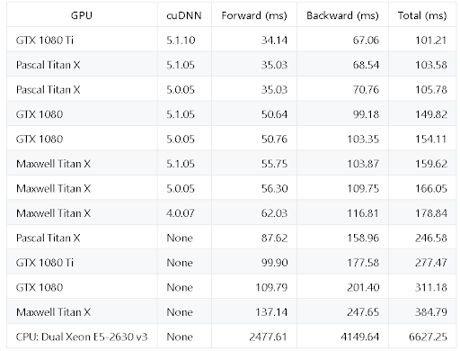
ResNet-50 Performance
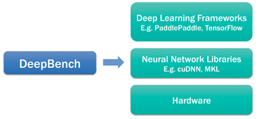
The DeepBench Platform from Baidu Research
Although the fundamental computations behind deep learning are well understood, the way they are used in practice can be surprisingly diverse. For example, a matrix multiplication may be compute-bound, bandwidth-bound, or occupancy-bound, based on the size of the matrices being multiplied and the kernel implementation. Because every deep learning model uses these operations with different parameters, the optimization space for hardware and software targeting deep learning is large and underspecified.
DeepBench attempts to answer the question, “Which hardware provides the best performance on the basic operations used for deep neural networks?” The primary purpose is to benchmark the core operations that are important to deep learning across a wide variety of hardware platforms.
They employ the following core operations to evaluate the competing hardware platforms:
Dense and sparse matrix multiplications
Convolutions: works for multiple approaches like direct, matrix multiply based, FFT based, and Winograd based techniques
Recurrent layer operations (support for three types of recurrent cells; vanilla RNNs, LSTMs, and GRUs)
All-reduce: Training efficiency across a set of parallelized GPUs, in both synchronous and asynchronous
The results are available on their Github repo in the form of simple Excel files.
Summary of Computer Vision (CV) Being Used in AI & ML Systems
In this article, we started with the characteristics and challenges associated with modern large-scale computer vision tasks, as aided by complex deep learning networks. The challenges can be well understood in the context of two of the most promising applications — autonomous driving and medical imaging.
We also went over the datasets, storage, and computing (GPU vs. CPU) requirements for the CV systems and discussed some key desirable features that this kind of system should possess.
Finally, we talked about a few open-source resources that benchmark hardware platforms for high-end deep learning/CV tasks and showed some key performance benchmark tables for popular hardware choices.
Computer vision will continue to advance in the coming years as breakthroughs in hardware and algorithms lead to new performance gains.
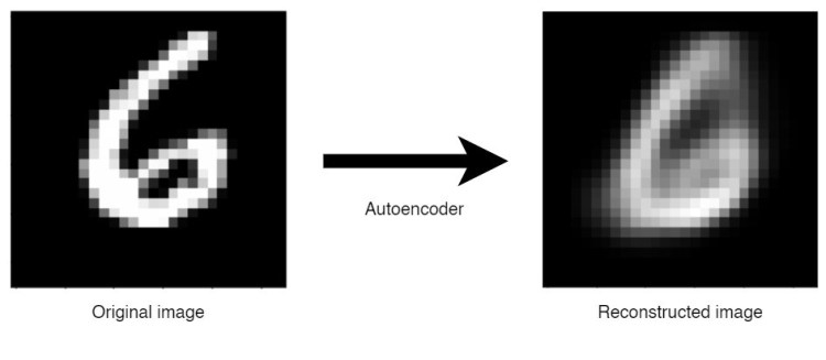
Deep Autoencoder in Action: Reconstructing Handwritten Digit
Image reconstruction using autoencoder.
Hello world, welcome back to my page! Here I wanna show you another project that I just done, A Deep Autoencoder. So autoencoder is essentially just a kind of neural network architecture, yet this one is more special thanks to its ability to generate new data based on given sample represented in lower dimension. Here I am going to be using MNIST Handwritten Digit dataset in which each of its image samples has the size of 28 by 28 pixels. This size is then going to be flattened, hence we will have 784 values to represent each of those images.
As usual, I also include all code required for this project in the end of this article.
Big Data Jobs
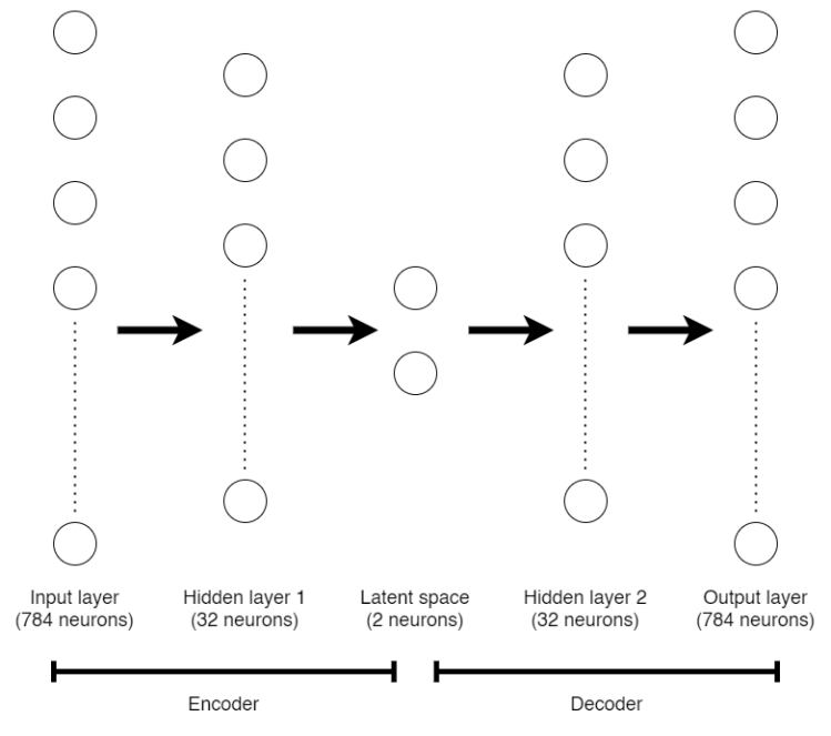
Before we jump into the code, let me explain first about the structure of a deep autoencoder. Look at the figure below.
Structure of the deep autoencoder used in this project.
What you are seeing in the picture above is a structure of the deep autoencoder that we are going to construct in this project. An autoencoder has two main parts, namely encoder and decoder. The encoder part, which covers the first half of the entire network, has a purpose to map a sample into its lower dimensional representation. In this case, the encoder consists of an input layer which takes 784 features. Next, it is connected to a hidden layer of 32 neurons and then followed by 2-neurons layer. The encoder part ends at this 2-neurons layer, which is usually called as latent space. Since this latent space has exactly two dimensions, then we are able to represent all the data in a simple cartesian coordinate system in order to find out where the location of those digit numbers are encoded.
The next half of an autoencoder is called decoder. The architecture of a decoder is nearly the same as the encoder part. However, instead of lowering the dimensionality of data, it maps back a value in latent space to the original image shape. In this project, the decoder takes two input values, in which it should be two coordinate numbers that represent a location in a latent space. Then it is attached to a hidden layer and output (original shape) layer of size 32 and 784 respectively.
I think that’s all of the explanation about autoencoder, so now let’s start to implement this!
As usual, the first thing to do is to import all required modules, namely NumPy, Matplotlib, and Keras. The MNIST Handwritten Digit dataset that we will use is available from Keras datasets, so we can load it directly through the code.
import numpy as np
import matplotlib.pyplot as plt
from keras.datasets import mnist
from keras.models import Model
from keras.layers import Dense, Input
Now that we already have 4 variables, where X_train and y_train consist of 60000 data-label pairs while the test variables consist of 10000 pairs. Spoiler alert: we do not use use both y_train and y_test for training. I will explain the reason later.
After loading the dataset, the next thing to do is to preprocess those data. Fortunately, the preprocessing steps is very simple for this case because the shape of the images are already uniform (28 by 28). So now, what we need to do is to flatten out both X_train and X_test, then keep those flattened array to X_train_flat and X_test_flat.
If we check the shape of both flattened variables you will get (60000, 784) and (10000, 784) for train and test data respectively.
The next preprocessing step is array values normalization. We know that pixel brightness in images are represented with values ranging between 0 and 255. In order for neural network to work best, we need those numbers to lie between 0 and 1, Even though in some other cases this step might not affect much. The normalization process can be done like this:
In addition, we do not convert both labels (y_train and y_test) into one-hotencoding representation because, as I said earlier, those data are literally not used to train the neural network model.
Constructing the autoencoder
After all preprocessing steps done, now we are able to construct the autoencoder. The structure of this deep autoencoder is already shown in the figure that I put in the early part of this writing. Below is the code implementation of the architecture.
Technically speaking, this deep autoencoder takes an array of size 784 as the input value (the flattened image array). Next, those values are delivered to the next layers, namely hidden_1, latent_space and hidden_2 respectively before eventually reach the last layer called output_1. Note that we call this a deep autoencoder due to the existence of hidden_1 and hidden_2 layer. If those two layers do not exist, we can simply call it as an autoencoder.
Next, we need to define the segments of the network (encoder, decoder, and the entire model). Here I will use a variable called autoencoder to store the entire neural network model and use encoder variable to store the first half of the network.
Notice the way I define the model variables. The autoencoder takes the very first layer (input_1) as the input and the very last layer (output_1) as the output in order to take all the 5 layers of the network. The encoder part, however, stops at the latent_space because we want to take the value from this layer to get the lower dimension representation of an image data.
The decoder part is kinda tricky though. Below is the code creating the decoder part:
First we need to create a placeholder called decoder_input. This is done because essentially we want to give a particular value as the input of the latent_space, while the latent_space itself is actually not an input layer. So we can say that decoder_input and latent_space are actually representing the same layer, but decoder_input takes a value from user while the latent_space takes a value from the previous layer of the network.
Next, I define more decoder layers which are also basically taken from the layers of the model stored in autoencoder variable. decoder_layer_1 is exactly the same as the second last layer of the entire network, while decoder_output is the same as the output of autoencoder. Lastly, we need to define the decoder variable itself which is the second half of the entire network.
We may check the entire structure of this deep autoencoder using autoencoder.summary() just to check whether we have already constructed the model exactly like what is displayed in the picture I shown earlier. Below is the model summary.
You may also run encoder.summary() or decoder.summary() if you want.
Compiling and fitting the model
A neural network can not be trained before we define the loss function and the optimizer. In this case, I decided to go with binary cross entropy loss function and adam optimizer. You may change this loss function to something like mse (Mean Squared Error), while other optimizers like adagrad or adadelta are also applicable. Below is how I compile the model:
Notice that when fitting (a.k.a. training) the neural network model, the first and second argument are the same variable (both are X_train_flat). If you are familiar with classification task, usually we set the first argument as the sample (X) while the second one is used to pass the ground truth (y). The reason why in autoencoder we pass both X variables is because we want the output of the model to be as similar as possible with the input data. Therefore, as I have mentioned in the earlier part of this writing, actually loading y_train and y_test is not necessary for the training process.
Anyway, below is the output of the model fitting after 10 epochs. We can see here that the loss value decreases as the epoch goes. Theoretically, this loss value can still go lower as we increase the number of epochs. Note that I removed the result of epoch 2 to 9 for simplicity.
Up to this point, our deep autoencoder has just been trained well. Now that we are able to find out the lower dimension representation of all images and draw the distribution in a simple scatter plot using encoder. Then we can also use the decoder to perform digit image reconstruction.
What’s done by encoder?
After training the entire deep autoencoder model, we can perform mapping from 784-dimension flattened image to 2-dimension latent space. Now we are going to try to map all those training data into latent space using only the encoder part of the model, which can be achieved using the following code:
encoded_values = encoder.predict(X_train_flat)
Here the shape of encoded_values variable is (60000, 2), where it represents the number of samples and its dimension respectively. We can think of this 2-dimensional shape as a value in x-y coordinate system for each sample. Hence, we are able to put all those data into a scatter plot. Notice that the y_train is used to color-code the samples. Below is the code to do so:
Digit samples represented in two-dimensional latent space.
And there it is! The figure above shows the handwritten digit distribution in two-dimensional latent space. Previously, each of the images in the dataset are represented in 784 dimensions, which is absolutely impossible to visualize the label distribution. However, now it is a lot easier to see the distribution of all images because we have encode those high data dimension to only 2 dimensions.
Furthermore, the scatter plot above tells some interesting facts. First, we can see that the picture with label 1 (orange) looks very far from most of the other images. Here we can say that images with label 1 are very different with most other numbers. Next, when we pay more attention to data points with label 4 and 9 (those in between pink and purple), we can say that these two handwritten digits are quite similar to each other due to the fact that these data points are literally spread in a same cluster.
That’s all of the encoder, now let’s jump into decoder.
What’s done by decoder?
Now, what if we are given a pair of x-y coordinate value representing a point in a latent space? Can we reconstruct the handwriting image from that point? Yes we can! It can simply be achieved by performing prediction using the decoder model that we defined earlier.
decoded_values = decoder.predict(encoded_values)
Remember, the shape of encoded_values variable is (60000, 2), meaning that it contains 60000 data points in our latent space in which each of those samples are represented using two values. Now we use this variable as the argument of predict() method on the decoder, in which its return value is a 60000 flattened images where each of those images are having 784 values representing the brightness of each pixel. Since the MNIST image should have the size of 28 by 28, then we still need to reshape this output value. Below is the code for it.
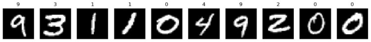
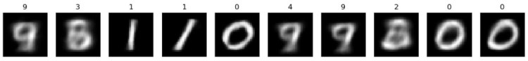
Up to this point, we already got the reconstructed images stored in decoded_values variable. Now we can compare each of the sample value stored in the variable with the actual handwritten digit image stored in X_train variable. Here I decided to print out 10 images of index 110 to 119 (out of 60000).
Below is the code to display the actual images taken from X_train and its output along with the labels:
# Display some images
fig, axes = plt.subplots(ncols=10, sharex=False,
    sharey=True, figsize=(20, 7))
counter = 0
for i in range(110, 120):
    axes[counter].set_title(y_train[i])
    axes[counter].imshow(X_train[i], cmap='gray')
    axes[counter].get_xaxis().set_visible(False)
    axes[counter].get_yaxis().set_visible(False)
    counter += 1
plt.show()
Actual images of index 110 to 119.
And the code below is used to display the reconstructed images, also with its ground truth.
# Display some images
fig, axes = plt.subplots(ncols=10, sharex=False,
    sharey=True, figsize=(20, 7))
counter = 0
for i in range(110, 120):
    axes[counter].set_title(y_train[i])
    axes[counter].imshow(decoded_values[i], cmap='gray')
    axes[counter].get_xaxis().set_visible(False)
    axes[counter].get_yaxis().set_visible(False)
    counter += 1
plt.show()
Reconstructed images of index 110 to 119.
Now we can compare some of the actual and reconstructed images pretty clearly. In fact, these reconstructed images are exactly like what I expected. Remember the latent space I displayed earlier. It shows us that data points with label 1 is clearly separated from nearly all other samples. This makes reconstructing the handwritten digit of 1 is pretty easy that it looks like there is no much noise generated in its reconstructed image. Next, for the case of number 4 and 9, as I explained earlier as well, it seems those two numbers are quite similar to each other due to the fact that in the latent space they are spread in the same cluster. We can also see the reconstructed images above that the number of 4 and 9 are kinda indistinguishable.
Don’t worry if you get different latent space image when trying to run the code by yourself since it also produces different results in my computer when I try to run it multiple times.
Thank you very much for reading! Hope you learn something new from this post!
Autonomous machines are already a significant feature of modern society and are becoming ever more pervasive. Although they bring undoubted benefits, this is accompanied by concerns.
It is important that such machines function as a benign part of our society, and this means that they should behave in an ethical manner. Conventional machines are required to meet safety standards, but autonomous machines additionally need to come with some assurance that their decisions are not harmful.
In this article we will talk about the current ethical theories and briefly describe them. We will consider three types of ethical theory: consequentialist approaches, deontological approaches, and virtue ethics approaches. The intention is certainly not to argue that one approach is better than another as an account of human ethics, but rather to explore the effects of adopting the various approaches when implementing ethical agents.
Big Data Jobs
Defining an ethical agent
First, let us define what an ethical agent is. Our notion of an ethical agent is an agent that behaves in a manner which would be considered ethical in a human being. This may be considered to be in the spirit of weakAI, and adapts Minky’s definition of AI which relates to activity produced by a machine that would have been considered intelligent if produced by a human being [1]. The agents in our discussion will not be expected to model or perform ethical reasoning for themselves, but merely to behave ethically. The approaches to ethics we discuss will belong to the system designers, not the agents, and we will be exploring the consequences of the designers adopting a particular approach to ethics on the agents they implement. This may result in the implemented agents representing a rather thin version of the approach they embody.
By adopting this relatively weak notion of what it means for an agent be ethical, we are able to exclude from consideration anything dependent on mental states, or motivation, and questions such as whether the ethics developed by an agent, whose needs and form of life greatly differ from those of humans, would be acceptable to humans. We believe that using this notion is not a problem: on the contrary ethical agents are needed now, and while weakly ethical agents are currently feasible, strongly ethical agents currently lie in the, perhaps distant, future.
Consequentialism
This approach holds that the normative properties of an act depend only on the consequences of that act. Thus whether an act is considered morally right can be determined by examining the consequences of that act: either of the act itself (act utilitarianism, associated with Jeremy Bentham, [2]) or of the existence a general rule requiring acts of that kind (rule utilitarianism, often associated with John Stuart Mill [3]). This gives rise to the question of how the consequences are assessed. Both Bentham and Mill said it should be in terms of the greatest happiness of the greatest number, although Mill took a more refined view of what should count as happiness.** However, there are a number of problems associated with this notion, and many varieties of pluralistic consequentialism have been suggested as alternatives to hedonistic utilitarianism.
Equally there are problems associated with which consequences need to be considered: the consequences of an action are often not determinate, and may ramify far into an unforeseeable future. However, criticisms based on the impossible requirement to calculate all consequences of each act for every person, are based on a misunderstanding. The principle is not intended as a decision procedure but as a criterion for judging actions: Bentham wrote It is not to be expected that this process [the hedonic calculus] should be strictly pursued previously to every moral judgment. [4]. Despite the difficulty of determining all the actual consequences of an act (let alone a rule), there are usually good reasons to believe that an action (or rule) will increase or decrease general utility, and such reasons should guide the choices of a consequentialist agent. This has led some to distinguish between actualism and probabilism. On the latter view, actions are judged not against actual consequences, but against the expected consequences, given the probability of the various possible futures. Given our notion of a weakly ethical agent, the agent itself will be supplied with a utility function, and will choose actions that attempt to maximise it. The choice of the utility function, and the manner in which consequences are calculated will be the responsibility of the designer.
Deontological ethics
The key element of deontological ethics is that the moral worth of an action is judged by its conformity to a set of rules, irrespective of its consequences. One example is the ethical philosophy of Kant [5]; a more contemporary example is the work of Korsgaard [6]. The approach requires that it is possible to find a suitable, objective, set of moral principles. At the heart of Kant’s work is the categorical imperative, the concept that one must act only according to that precept which he or she would will to become a universal law, so that the rules themselves are grounded in reason alone. Another way of generating the norms is offered by Rawl’s Theory of Justice [7], in which the norms correspond to principle acceptable under a suitably described social contract. The principles advocated by Scanlon in [8] are those which no one could reasonably reject. Divine commands can offer another source of norms to believers. Given our weak notion of an ethical agent which requires only ethical behaviour, the rules to be followed will be chosen by the designer, and the agent itself will be a mere rule follower. Thus the agent itself will embody only a very unsophisticated part of deontology: any sophistication resides in the designer who develops the set of rules which the agent will follow.
Problems of deontological ethics include the possibility of normative conflicts (a problem much addressed in AI and Law, e.g. [9]) and the fact that obeying a rule can have clearly undesirable consequences. Many are the situations when it can be considered wrong to obey a law of the land, and it is not hard to envisage situations where there are arguments that it would be wrong to obey a moral law also. Some of this may be handled by exceptions (which may be seen as modifications which legitimize violation of the general rule in certain prescribed circumstances) to the rules. Exceptions abound in law and their representation has been much discussed in AI and Law: for example exceptions to the US 4th Amendment in, e.g. [10] and [11]. Envisaging all exceptions, however, is as impossible as foreseeing all the consequences of an action. For this reason laws are often couched in vague terms (reasonable cause and the like) so that particular cases can be decided by the courts in the light of their particular facts. This will mean that whether the rule has been followed or not may require interpretation.
Virtue Ethics
Virtue ethics is the oldest of the three approaches and can be traced back to Plato, Aristotle and Confucius. Its modern re-emergence can be found in [12]. The basic idea here is that morally good actions will exemplify virtues and morally bad actions will exemplify vices. Traditional virtue ethics are based on the notion of Eudaimonia [13], usually translated as happiness and flourishing. The idea here is that virtues are traits which contribute to, or are a constituent of, Eudaimonia. Alternatives are; agent based virtue ethics, which understands rightness in terms of good motivations and wrongness in terms of the having of bad (or insufficiently good) motives [14], target centered virtue ethics [15], which holds that we already have a passable idea of which traits are virtues and what they involve, and Platonist virtue ethics, inspired by the discussion of virtues in Plato’s dialogues [16] . There is thus a wide variety of flavors of virtue ethics, but all of them have in common the idea that an important characteristic of virtue ethics is that it recognizes diverse kinds of moral reasons for action, and has some method (corresponding to phronesis (practical wisdom) in ancient Greek philosophy) for considering these things when deciding how to act. Because there are few exemplars of implementations using the virtue ethics approach in agent systems, we will provide our own way of implementing a version of virtue based ethics in an agent system, based on value-based practical reasoning [17] , which shows how an agent can choose an action in the face of competing concerns. The various varieties of virtue ethics do, of course, have a lot more to them, but again, given that we are considering weakly ethical agents, these considerations and the particular conception of virtue will belong to the designers, who will implement their agents to behave in accordance with their notions of virtuous behavior, through the provision of a procedure for evaluating competing values.
** Mill wrote in [45] “It is better to be a human being dissatisfied than a pig satisfied; better to be Socrates dissatisfied than a fool satisfied.” Bentham, in contrast stated “If the quantity of pleasure be the same, pushpin is as good as poetry.”
1. M. Minsky, Semantic Information Processing, MIT Press, 1968
2. J. Bentham, The Rationale of Reward, John and HL Hunt, 1825
3. J.S. Mill, Utilitarianism, Longmans, Green and Company, 1895
4. J. Bentham, The Rationale of Reward, John and HL Hunt, 1825.
5. I. Kant, The Moral Law: Groundwork of the Metaphysics of Morals, first published 1785, Routledge, 2013.
6. C.M. Korsgaard, The Sources of Normativity, Cambridge University Press, 1996.
7. J. Rawls, A Theory of Justice, Harvard University Press, 1971.
8. T. Scanlon, What We Owe to Each Other, Harvard University Press, 1998.
9. H. Prakken, Logical Tools for Modelling Legal Argument, Kluwer Law and Philosophy Library, Dordrecht, 1997.
10. T. Bench-Capon, Relating values in a series of Supreme Court decisions, in: Proceedings of JURIX 2011, 2011, pp. 13–22.
11. T. Bench-Capon, S. Modgil, Norms and extended argumentation frameworks, in: Proceedings of the Seventeenth International Conference on Artificial Intelligence and Law, ACM, 2019, pp. 174–178.
12. G.E.M. Anscombe, Modern moral philosophy, Philos. 33 (124) (1958) 1–19.
13. H. Rackham, Aristotle. The Eudemian Ethics, Harvard University Press, Cambridge, 1952.
14. M. Slote, The Impossibility of Perfection: Aristotle, Feminism, and the Complexities of Ethics, OUP USA, 2011.
15. C. Swanton, Virtue Ethics: A Pluralistic View, Clarendon Press, 2003.
17. K. Atkinson, T. Bench-Capon, Practical reasoning as presumptive argumentation using action based alternating transition systems, Artificial Intelligence, 171 (10–15) (2007) 855–874.
If you liked this article, please feel free to clap for it. You can contact me through LinkedIn; I am always ready to have a meaningful conversation. If you want to keep reading the articles, I write, please hit the follow button. You will be notified when I publish an article.
Data science work typically requires a big lift near the end to increase the accuracy of any model developed. These five recommendations will help improve your machine learning models and help your projects reach their target goals.
In this article, we will focus on various machine learning, deep learning models, and applications of AI which can pave the way for a new data-centric era of discovery in healthcare.


