365 Data Science is an online educational career website that offers the incredible opportunity to find your way into the data science world no matter your previous knowledge and experience.
New Poll: What Python IDE / Editor you used the most in 2020?; Automating Every Aspect of Your Python Project; Autograd: The Best Machine Learning Library You’re Not Using?; Implementing a Deep Learning Library from Scratch in Python; Online Certificates/Courses in AI, Data Science, Machine Learning; Can Neural Networks Show Imagination?
Getting started in deep learning – and adopting an organized, sustainable, and reproducible workflow – can be challenging. This blog post will share some tips and tricks to help you develop a systematic, effective, attainable, and scalable deep learning workflow as you experiment with different deep learning models, datasets, and applications.
The latest KDnuggets polls asks which Python IDE / Editor you have used the most in 2020. Participate now, and share your experiences with the community.
Hi! Ardi here. In my previous post I was writing about the statistical approach to solve linear regression problem, which is basically only using several formulas to create a best-fit straight line to estimate the value of dependent variable y based on given training data x. Click the link below if you wanna read the article.
Today, in this post I wanna do the similar thing, yet this one is going to be done using machine learning approach. In statistics, we do not use optimization algorithm to solve this task. On the other hand, such algorithm is required in the field of machine learning. Here I decided to use gradient descent optimization algorithm (which is the simplest one) to minimize the value of MSE (Mean Squared Error). Furthermore, the dataset I use in this project is exactly the same as what I use in the previous post, which can be downloaded from here.
Machine Learning Jobs
Note: I put the full code at the end of this post.
Now let’s start to load the required modules first:
import numpy as np
import pandas as pd
import matplotlib.pyplot as plt
As you can see here we do not import Sklearn module since we are going to do all the calculation from scratch.
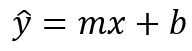
Before we go deeper into the machine learning, it’s important to know that the linear regression line is basically just a linear function — hence the name is linear regression. The equation can be denoted like this:
Linear regression equation.
Here x is used to represent all samples in the dataset. Notice that here I use y_hat (instead of just y) since the line basically represents value predictions, not the actual target value. The main objective of doing linear regression is to figure out the value of m and b, which represent slope and y-intercept respectively. In statistical approach, we can directly apply a formula to compute those unknown values. However, here in machine learning, we are going to start by assigning random value for both variables and then we try to predict the best value for m and b with the help of error/loss function and optimization algorithm. Basically the idea here is to use optimizer to minimize the error value gradually.
Now let’s load our dataset and check how the distribution looks like.
df = pd.read_csv('student_scores.csv')
df.head()
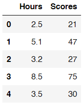
How our dataset looks like.
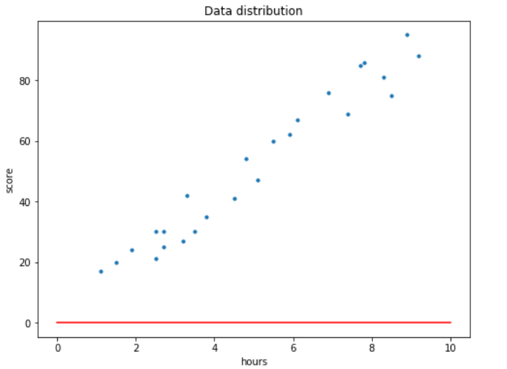
So our dataset here consists of 2 columns, namely Hours and Scores. Those columns essentially show the students’ studying duration and the score they obtain in final exam respectively. The goal of this task is to predict students’ final exam score based on their studying duration. Hence, we can say that values in Hours column is going to be our independent variable x, while numbers in Scores column will be our dependent variable y. To make things look more straightforward, here I assign the values in both columns to array x and y.
x = df['Hours'].values
y = df['Scores'].values
Now we can use plt.scatter() to see how the distribution looks like.
plt.figure(figsize=(8,6))
plt.title('Data distribution')
plt.scatter(x, y, s=30)
plt.xlabel('hours')
plt.ylabel('score')
plt.show()
How the data distribution looks like.
Loss function: MSE (Mean Squared Error)
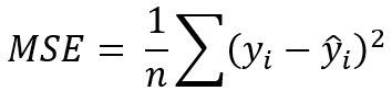
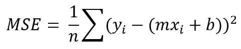
Before doing the error minimization process, we have to know first how our error function looks like. Here I decided to use what’s called as MSE.
Mean Squared Error loss function.
The function above is pretty simple though. Here y, y_hat and n represent actual y, predicted y and the number of samples in our dataset. Also, it’s important to remember that i denotes i-th sample. Next, since the prediction y_hat is essentially obtained using our regression line, then we can substitute this variable with a linear function.
Plugging y_hat equation to MSE.
Still, our problem here is that we do not have the optimal value for m and b just yet such that the error value is minimized. So in the next step we are going to use gradient descent algorithm to gradually update this m and b values.
Gradient descent algorithm
There are several steps that we need to do to run this algorithm:
First: initialize value for m and b. I mentioned earlier that the value of these 2 variables should be random numbers. However, to make things simpler, I decided to assign 0 to both variables as the initial value.
m = 0
b = 0
If we try to print our line with m=0 and b=0, then we are going to see an output like this:
x_line = np.linspace(0,10,100)
y_line = m*x_line + b
Second: define learning rate L and number of epochs. In simple words, learning rate defines how fast our gradient descent algorithm reduces error value for each epoch (iteration). Generally, the value of learning rate is a very small number. Here I decided to set the the value to 0.001. It’s important to keep in mind that small L value slows down the training process (we might need to increase the number of epochs), yet on the other hand, large learning rate value may cause our gradient descent algorithm fail to reach its minimum error.
L = 0.001
epochs = 100
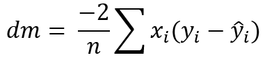
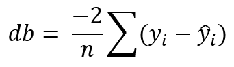
Third: calculate the partial derivative of our loss function with the respect to m and b. Here I store those derivatives to dm and db.
Derivative of MSE with the respect of m.Derivative of MSE with the respect of b.
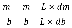
Fourth: update the value of m and b by taking into account the value of both derivatives and learning rate. Note that the third and fourth step are going to be done iteratively.
Updating the value of m and b.
Implementation
As we already got the idea of how gradient descent algorithm works, now we can start to implement this in the code. All the code below are based on the mathematical notations we defined earlier.
# The number of samples in the dataset
n = np.float(x.shape[0])
# An empty list to store the error in each epoch
losses = []
for i in range(epochs): yhat = m*x + b
# Keeping track of the error decrease mse = (1/n) * np.sum((y - yhat)**2) losses.append(mse)
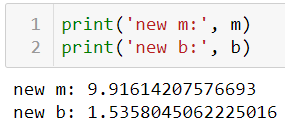
After the training process is done, we can try to print out the new value of m and b. We can see here that now those values have been updated thanks to the gradient descent algorithm.
New values of m and b after 100 epochs.
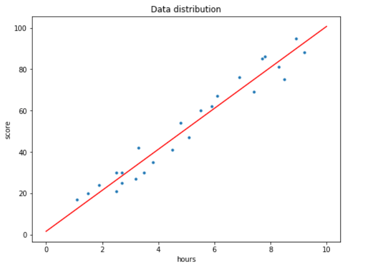
If we display the regression line with these updated values, we should get the following output:
x_line = np.linspace(0,10,100)
y_line = m*x_line + b
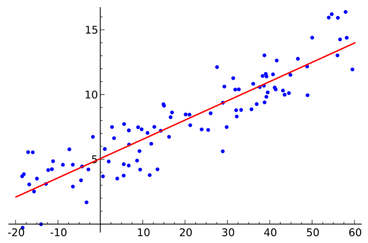
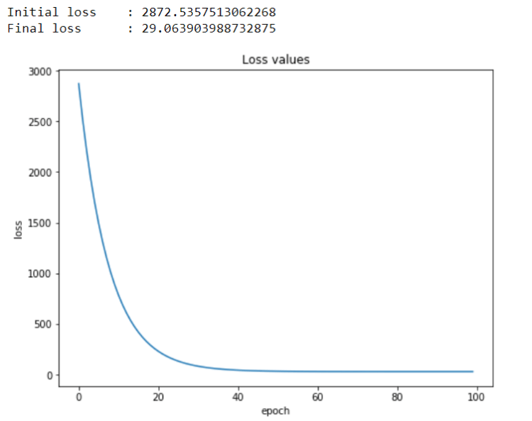
We can see here that our algorithm works well as it’s now able to create a line which approximates all data points in our dataset. In other words, we can also say that this regression line produces much smaller error compared to our initial line when m = b = 0. Here’s the code if you want to see how the error value decreases as the training process goes.
As product dealines are shrinking and software is growing only more and more sophisticated, companies are forced to introduce viable innovations into their SDLC to keep in step with market requirements and competitors. Quality assurance is a process rather notorious for being high-load, repetitive, and time-consuming but, at the same time, hugely important for the application’s overall success. Obviously, this is a primary candidate for streamlining with automation.
Today, QA automation is accorded high priority by software development teams. According to the recent ResearchAndMarket report, the global market for automated testing services and solutions is forecasted to grow from $12.6 billion in 2019 to $28.8 billion by 2024, with functional QA being the segment with the highest investment over the projected period. The increased demand has also set the stage for unprecedented quality improvements in test automation, as companies are turning to the emerging technologies to revamp their practices.
Among all the budding software testing innovations, machine learning (ML), a subset of AI, appears to be the most promising. The technology can train itself on historical data to create and maintain test cases, offering to go beyond the conventional rule-based automation that partially relies on the testing engineer’s manual efforts. Let’s explore what’s on the horizon for ML in software testing, touching upon the technology’s proven use cases and its transformative effect on the QA and software delivery.
Machine Learning Jobs
Visual validation in GUI testing
An algorithm might be unable to turn a canvas into a masterpiece, but it is already advanced enough to detect a masterpiece’s flaws — all due to computer vision. The technology that trains computers to properly understand and interpret visual objects can be successfully retrofitted to detect bugs, inconsistencies, and excessiveness in a user interface design.
To produce results, an ML testing algorithm first needs to learn from large sets of interface imagery where page elements are labeled, and good practices are distinguished from bad ones. As the system matures, it will be able to independently seek out faults in the software. To allow it to run end-to-end evaluation without constant supervision, such a computer vision-based solution is commonly equipped with a script that helps it move from page to page.
Although only nascent, computer vision QA automation is currently the focus of intense research, and standalone ML-powered solutions (Applitools is a prime example) already start appearing on the market.
Predictive test maintenance and self-healing in functional testing
Another key area of QA automation is functional testing. It is unsophisticated yet high-volume and repetitive, that’s why it’s rather taxing when performed manually. The commonly used coding automation substantially accelerates test execution but, on the other hand, requires continuous maintenance, such as for debugging and rewriting test cases that fail, tailoring them to altered conditions. Meanwhile, machine learning has all the prerequisites to resolve this limitation and fine-tune functional testing even further.
Predictive maintenance is an ML-enabled technique that recognizes failure patterns based on historical data. When implemented in an automated functional testing workflow, it will run an ongoing evaluation of the environment and identify changes that may destabilize test execution before it happens. Apart from this, artificial intelligence can power self-healing mechanisms by detecting the root issue of a failed test and promptly fixing it. This way, the recovery takes much less time than when done by a testing engineer, allowing for almost uninterrupted testing.
Test case modeling and generation in performance testing
Performance testing is an essential step in preparing for software release, as it helps ensure unfaltering operation at all times. Since it would require much effort to create an appropriate environment manually, partial automation has become a viable option for this testing type. A wealth of dedicated tools on the market allow generating real-life and extreme conditions and measure application performance. But machine learning can change the game here.
For one thing, it can prove extremely useful for test case creation. Geared towards pattern recognition, the algorithm runs an end-to-end system analysis, identifies weak points, and models test cases to address these deficiencies. Moreover, machine learning can take over the task of creating test scripts. Driven by Natural Language Processing, the algorithm can not only generate code but also fix any occurring issues, thus allowing software creators to fully focus on more creative tasks.
Today, more and more performance testing and monitoring tools are being retrofitted with AI/ML technologies, with such well-reputable solutions as AIMS, BMC Software APM, and Dynatrace among them.
Test scenarios planning and HIG assessment in mobile app testing
With the rapid growth of smartphone usage over the last decade, the mobile application market is forecasted to have a staggering CAGR of 19.2% in the next three years, as reported by Allied Market Research. In the context of such a high demand, development companies began relying on up-and-coming solutions to accelerate their SLDC, and machine learning became the top choice for many.
In an average mobile app QA project, planning and creating individual test scenarios take up a lot of time, yet involving machine learning and artificial intelligence is poised to automate these strategic steps. Analyzing an app from end to end, the algorithm can come up with the most suitable test cases and even execute the easiest ones.
Beyond that, ML can automate assessment against the Human Interface Guidelines (HIG) — the process that takes days for human reviewers. Trained on the HIG requirements, the tool can ‘walk’ through an application’s pages and seek out violations, helping the team meet their release deadlines.
To sum up
Machine learning has only begun making a difference in the software testing field, but the potential it holds for QA automation and DevOps is already promising. Implemented into the CI/CD pipeline, the technology will allow testing teams to not only accelerate bug detection and risk assessment but also make these processes smarter, error-free, and future-proof.
The growing interest in ML-QA integration has been lately raising the testing community’s concerns, as some fear being displaced by the more high-performing algorithms. Although the chances are high that the popularization of ML-powered testing will entail the establishment of higher standards for testing qualifications, in the foreseeable future, the technology is unlikely to become autonomous and self-sufficient enough to make the job disappear completely.
If you are looking for a machine learning starter that gets right to the core of the concepts and the implementation, then this new free textbook will help you dive in to ML engineering with ease. By focusing on the basics of the underlying algorithms, you will be quickly up and running with code you construct yourself.
Predictive analytics isn’t just for white-collar work. Check out these five examples that show its potential in blue-collar jobs and industries as well.
If EDA is not executed correctly, it can cause us to start modeling with “unclean” data. See how to use Pandas Profiling to perform EDA with a single line of code.
Hello world, this is Ardi! So in this writing I wanna show you how to construct a Neural Network using both sequential and functional model. As far as I know most of Neural Network tutorials out there are using sequential model, probably because it is more intuitive for simple architectures, even though in fact Functional model is actually not that complicated.
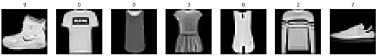
Here is my plan for this article: I will be using Fashion MNIST dataset which consists of 60000 train data and 10000 test data, in which each of those images have the size of 28 by 28 pixels (similar to MNIST Digit dataset). Next, two exact same classifier model will be created and trained. The first one is done using sequential style while the second one is using functional style. Lastly I will explain a bit why it is important to get familiar with functional style, especially if you’re interested to learn more about Neural Network-based models. So that’s it, let’s start doing this little project.
Note: scroll to the last part of this writing to get the fully-working code.
As usual, the first thing to do is to import all required modules. Notice that the Fashion MNIST dataset is already available in Keras, and it can just be loaded using fashion_mnist.load_data() command.
import numpy as np
import matplotlib.pyplot as plt
from keras.utils import to_categorical
from keras.datasets import fashion_mnist
from keras.models import Sequential, Model
from keras.layers import Dense, Input
for i in range(7):
    axes[i].set_title(y_train[i])
    axes[i].imshow(X_train[i], cmap='gray')
    axes[i].get_xaxis().set_visible(False)
    axes[i].get_yaxis().set_visible(False)
Artificial Intelligence Jobs
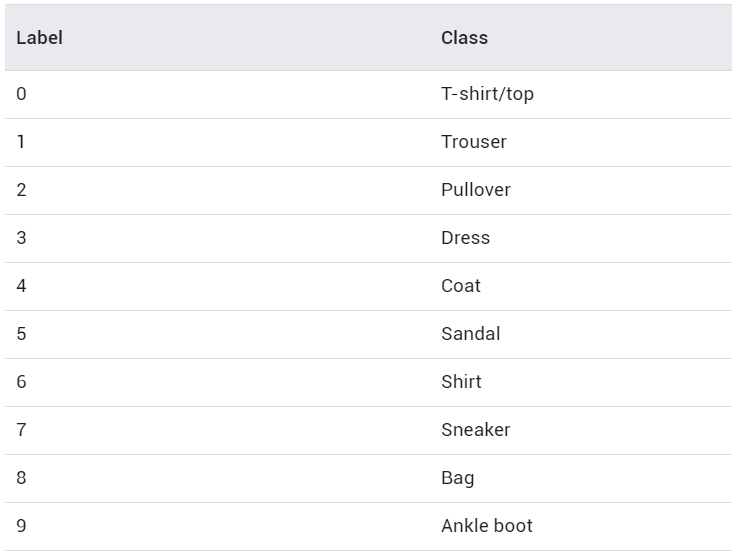
After running the code above, you should get an output of the first 7 images in the dataset along with the labels. As you can see the image below, those labels are already mapped to a particular number. If you check Keras documentation, you will be able to find out what those numbers actually mean (I also display it below).
Let’s get back into our X variables. Initially, each of the images stored in X_train and X_test is in form of 2-dimensional array with the shape of (28, 28), in which this size represents the height and width of the handwritten digit images. Before training the model, we need to flatten all those images first. It can be achieved by using NumPy reshape() function. The argument passed in this function represents the new shape that we want, in this case it’s (number of data, 28*28).
After running the code above, our X_train and X_test should have the shape of (60000, 784) and (10000, 784) respectively. Next, we also need to turn the target label (both y_train and y_test) into one-hot format. Use the following code to do that:
# Convert label to one-hot representation
temp = []
for i in range(len(y_train)):
    temp.append(to_categorical(y_train[i], num_classes=10))

y_train = np.array(temp)
temp = []
for i in range(len(y_test)):
    temp.append(to_categorical(y_test[i], num_classes=10))
y_test = np.array(temp)
Up to this stage we have already converted all train and test data along with its labels into the correct shape for our Neural Network model. So now we can start to construct the model architecture, I will start with Sequential model first.
Sequential Model
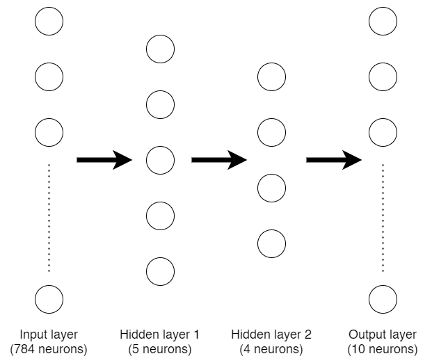
Architecture that we will construct for both sequential and functional model.
The first thing to do when we are about to create a sequential model is to initialize it first. The code below shows that we are initializing a new model called model_seq.
model_seq = Sequential()
Initially, this model_seq variable is just an empty Neural Network model until we add more layers sequentially starting from the beginning. Now I wanna create a Neural Network architecture like the one drawn in the figure above. To add layers into the model, we can use the following code.
The first layer that we add to model_seq is a dense (a.k.a. fully-connected) layer with 5 neurons. Keep in mind that the first layer added in a sequential model is not the input layer, it is our first hidden layer instead. The input layer is defined using input_shape argument, in this case I passed the shape of X_train variable which has the value of 784 (this is the number of our flattened image pixels).
Next, I add more hidden layer which consists of 4 neurons and an output layer of 10 neurons. Remember that we have 10 labels for this classification problem, so we need to use 10 neurons as well for the output layer.
Now since we already done constructing the architecture, we can print out the summary of the model simply by using model_seq.summary() command which directly gives output like this:
After that, we can compile and train the model using our X_train and y_train data pairs. I decided to use categorical cross entropy loss function and Adam optimizer with 3 epochs.
That’s the end of the training process on sequential model. You might notice that the accuracy is very low and at the same time the loss is very high, but it’s not the point of this writing! Here I just wanna show you how to construct a Neural Network using sequential and functional style.
So now let’s talk about the next one.
Functional Model
Functional model offers more flexibility because we don’t need to attach layers in sequential order. The code below shows the steps of creating the exact same model in functional way.
The first thing to do is to create the input layer, here I use input1 variable to define it. Also, don’t forget to pass the initial shape, in this case I use the shape of our X_train we defined earlier which has the size of 784 neurons.
In the next line, I create another variable namely hidden1 as the first hidden layer. Notice that I use dense layer with 5 neurons (exactly the same as our sequential model). To attach this layer with the input layer, we need to explicitly write input1 variable in the end of this line. After that, I define hidden2 as the second hidden layer which has 4 neurons and connects it to hidden1 using the same method. The last layer I wanna create in this model is the output layer with 10 neurons which connects to hidden2 layer.
Now, the final step of using functional style is to initialize the entire architecture. It can be achieved using Model() function along with its parameters which defines the input and output layer.
model_func = Model(inputs=input1, outputs=output)
Up to this stage we have already had two exact same Neural Network model. The first one was done previously using sequential style, while this one we just done it using functional style. When we run model_func.summary(), we will get the following output:
If we pay attention to the initial layer summary of both sequential and functional model, we will see that the input layer is not written in our sequential model. But this is completely fine as this input layer does not contain any params (weights), and hence does not affect the total number of params. You can see that in this case both models have 3999 params.
Next, we can continue to compile and train the model using the same procedure as the sequential model:
Again, I don’t really care about the accuracy and loss value for now. But, if you do care about it, you may increase the number of layers, neurons or epochs. Theoretically those things may help improving model accuracy.
So that’s it, now that you should be able to construct a Neural Network using both sequential and functional style. Personally, I prefer to use sequential style because most of the tutorials were using this kind of style when I started to learn implementing Neural Network, and I’ve been really comfortable with it until now. However though, it is also important to know how to do it using functional style since you can get more flexibility. For example, in sequential model you can only stack one layer after another, while in functional model you can connect a layer to literally any other layer.
Thanks for reading! I hope this article makes you learn something new!
And here is the entire code used in this project 🙂