365 Data Science

A review outside the common datasets for Machine Learning

When you being in the Machine Learning field, you usually use the common datasets such as MNIST, Iris, the 20 newsgroups, … But there are hundreds of rare and interesting datasets that can be found online. At Immune Technology Institute we have asked our teachers to create a list of the most strange datasets they have found. Here we go!!

Price of Weed

This is a repository which contains a registry of the historical marijuana prices, which shows significant differentiation at the state level in prices. The question here is how the data has been collected?

Although it may seem a useless dataset, it may be very relevant in the times we live in, as many countries are considering legalizing marijuana.

Length of chopsticks

If you have never asked you, as is normal, what is the optimal length of chopsticks, no worries, someone has asked this question before. A researcher team tried to evaluate the effects of the length of the chopsticks on the food-serving performance of adults and children. For this reason, they created this dataset for finding the optimal length of chopsticks.

They concluded that the food-pinching performance was considerably affected by the length of the chopsticks. The researchers suggested that families with children should provide both 240 and 180 mm long chopsticks. In addition, restaurants could provide 210 mm long chopsticks, considering the trade-offs between ergonomics and cost.

Rice Images

A dataset which contains more than of 3500 rice grain’s images of 2 different species. Different properties were extracted from each grain of rice, such as:

• The longest line that can be drawn on the rice grain
• The shortest line that can be drawn on the rice grain
• Or the perimeter of each grain.

Popular dog names in Sweden

Did you know that the most popular dog name in Sweden is Molly?

Sweden: popular dog names, by number of animals 2018 | Statista

This dataset collects the most popular dog names in Sweden in 2018 by number of animals. Bella ranked the second most popular name, with almost six thousand animals, followed by the name Charlie, reaching a number of approximately 4600.

Flags Data Set

I am pretty sure that Sheldon will love this one… This dataset contains details of various nations and their flags, such as:

• The religion of each country.
• The predominant colour in the flag.
• If the flag contains a crescent moon or sunstars.
• If it contains an eagle, a tree, …

Maybe it is interesting for predicting the religion of a country from its size and the colours in its flag.

Trending AI Articles:

1. Microsoft Azure Machine Learning x Udacity — Lesson 4 Notes

2. Fundamentals of AI, ML and Deep Learning for Product Managers

3. Roadmap to Data Science

4. Work on Artificial Intelligence Projects

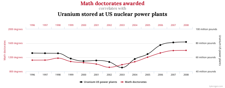
Sometimes it is also interesting to see how people find relationships in data where they are not visible to the naked eye. This website is an expert in finding correlations where no one else can find them, for example:

Cheese consumption vs Number of people who died by becoming tangled in their sheets

Math doctorates awarded vs Uranium stored at US nuclear power plants

Total revenues generated by arcades vs Computer science doctorates awarded in the US

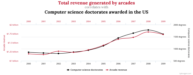
Discover new correlations using this website and share your results with us! ?

Discover a correlation

Who we are?

At Immune Technology Institute we try to apply and teach the most advanced technology at the computational field. Furthermore, we love sharing knowledge since we consider that it is when it becomes powerful.

If you want to learn how to develop real-world applications or how to handle large amounts of data, you could be interested in our Master in Data Science. It is a program aimed at professionals that seek to specialize in Data Science, know the main Artificial Intelligence techniques and how to apply them into different industries.

We will host an online information session on September 24, with the director of the master, Mónica Villas. IMMUNE can help you boost your career through its partner companies and contacts with recruiters and professionals in the sector. You can sign up HERE.

Wait one more thing — Datathon

Do you want to be a data scientist? Sign up for the virtual Datathon organized by IMMUNE Technology Institute in collaboration with Spanish Startups on September 19th. Online training from the best data experts and a great challenge to test your knowledge. Don’t miss out on the prize! You can sign up HERE.

This article have been written by: Alejandro Diaz Santos — (LinkedIn, GitHub) for IMMUNE Technology Institute.

Don’t forget to give us your ? !

---

A little bit of strange/interesting Datasets for Machine Learning was originally published in Becoming Human: Artificial Intelligence Magazine on Medium, where people are continuing the conversation by highlighting and responding to this story.

Via https://becominghuman.ai/a-little-bit-of-strange-interesting-datasets-for-machine-learning-8c76d8112cf?source=rss—-5e5bef33608a—4

Via https://becominghuman.ai/whats-so-trendy-about-open-source-social-media-apis-that-everyone-went-crazy-over-it-983d9920135?source=rss—-5e5bef33608a—4

Looking at data one way can tell one story, but sometimes looking at it another way will tell the opposite story. Understanding this paradox and why it happens is essential, and new tools are available to help automatically detect this tricky issue in your datasets.

Originally from KDnuggets https://ift.tt/33AK4Ls

In this article, we will look at the difference between generative and discriminative models, how they contrast, and one another.

Originally from KDnuggets https://ift.tt/32FC9x6

Coursera’s Machine Learning for Everyone (free access) fulfills two different kinds of unmet learner needs, for both the technology side and the business side, covering state-of-the-art techniques, business leadership best practices, and a wide range of common pitfalls and how to avoid them.

Originally from KDnuggets https://ift.tt/33H9Q0w

Everybody knows how important is understanding your customer, but how to do that in an era of Information Overload?

Originally from KDnuggets https://ift.tt/33F4HWO

Data Science the smart way: Regression — Part II

We are continuing our series on Data Science the smart way. This series helps you to master data science smartly through questions which is beneficial for concept clearance and interview preparation.

You can visit the first part of the blog here.

We have discussed questions about the regression in our first part of this blog. You can check the blog here. We have collected a brilliant set of questions from here.

Today we will discuss the following questions in detail. I will rate the questions as per their difficulty level.

• What are the methods for solving linear regression do you know? ‍[Medium]
• What is the normal equation? ‍[Medium]
• What is gradient descent? How does it work? ‍[Medium]
• What is SGD — stochastic gradient descent? What’s the difference with the usual gradient descent? ‍[Medium]
• Which metrics for evaluating regression models do you know? [Easy]
• What are MSE and RMSE? [Easy]

Let’s get started.

1. What are the methods for solving linear regression do you know?

There are many different methods used to solve the linear regression problem. We would discuss a few here.

i. Sklearn’s Linear Regression

ii. Gradient Descent

iii. Least Square Method/Normal Equation Method

iv. Singular Value Decomposition (SVD).

i. Sklearn’s Linear Regression

Linear Regression is a regression technique, falls in the category of supervised learning in machine learning. Linear regression is a predictive analysis technique that generally finds the relationship between the dependent variable and the independent variable. We visualize it by plotting the dependent(x-axis) and independent(y-axis) variables in 2D graph.

The implementation of Linear Regression using Sklearn is quite simple.

from sklearn.linear_model import LinearRegression
lr = LinearRegression()
lr.fit(X,y)

lr.intercept_, lr.coef_
(array([4.21509616]), array([[2.77011339]]))

lr.predict(X_new)
array([[4.21509616],[9.75532293]])

ii. Singular Value Decomposition (SVD)

The linear regression class is based on the scipy.linalg.lstsq() function (the name stands for “least squares”).

theta_best_svd, residuals, rank, s = np.linalg.lstsq(X_b, y, rcond=1e-6)
>>> theta_best_svd
array([[4.21509616],
[2.77011339]])

The function computes:

Where X^+ is the pseudoinverse of X. The pseudoinverse is computed using a standard matrix factorization technique called the singular vector Decomposition (SVD) that can decompose the training et matrix X into the matrix multiplication of three matrices U Σ V⊺. The decomposition helps in matrix multiplication if it is not invertible.

This approach is more efficient than computing the Normal equation, plus it handles edge cases nicely. The normal equation may not work if the matrix X⊺X is not invertible(i.e., singular), such as if m<n if some features are redundant, but the pseudoinverse is always defined.

Lets now see the implementation:

np.linalg.pinv(X_b).dot(y)
array([[4.21509616], [2.77011339]])

2. What is the normal equation?

Before explaining the normal equation. Let’s understand in short how does linear regression works.

A linear model makes a prediction by simply computing a weighted sum of the input features, plus a constant called the bias term (also called intercept term).

In this equation:
• ŷ is the predicted value.
• n is the number of features.
• xi is the ith feature value.
• θj is the jth model parameter (including the bias term θ0 and the feature weights
θ1, θ2, ⋯, θn)

This can be written in the vectorized form:

• θ is the model’s parameter vector, containing the bias term θ0 and the feature weights θ1 to θn.
  • x is the instance’s feature vector, containing x0 to xn, with x0 always equal to 1.
  • θ · x is the dot product of the vectors θ and x, which is of course equal to θ0x0 + θ1×1 + θ2×2 + … + θnxn.
  • hθ is the hypothesis function, using the model parameters θ

We know that to find the performance of the regression problem we minimize the MSE, RMSE.

The MSE of a Linear Regression hypothesis hθ on a training set X is calculated using:

Normal Equation:

To find the value of θ that minimizes the cost function, there is an equation that gives results directly. This is called the normal equation.

In this equation:
• θ is the value of θ that minimizes the cost function.
• y is the vector of target values containing y(1) to y(m).

3. What is gradient descent? How does it work?

Gradient Descent is a generic optimization algorithm that is used to finding an optimal solution to a wide range of problems. In Gradient Descent we tweak parameters iteratively in order to minimize the code function.

Suppose its raining in a hill. The water would flow towards the slope to the ground below. That’s what exactly gradient descent does: It measures the local gradient of the error function with regards to the parameter θ, and it goes to the direction of the descending gradient. Once the gradient is zero, we reach the minimum spot.

In the above picture of gradient descent, the model parameters are initialized randomly and get tweaked repeatedly to minimize the cost function; the learning step size is proportional to the slope of the cost function. The steps gradually get smaller and smaller as the parameters approach the minimum.

The important parameter in GD is the size of the steps, determined by the learning rate hyperparameter. If the learning rate is too small, then the algorithm will have to go through many iterations to converge, which will take a long time. On the other hand, if the learning rate is too high, you might jump across the valley and end up on the other side.

4. What is SGD — stochastic gradient descent? What’s the difference with the usual gradient descent?

Firstly we would understand what is Batch Gradient Descent then we will learn the Stochastic gradient descent.

To implement gradient descent we need to calculate how much the cost function will change if you change θj just a little bit. This method is called the partial derivative.

The partial derivative of the cost function is given by the equation. Note this is for a single case.

Instead of computing these partial derivatives individually, we can compute all of them in one go. The following equation contains all the partial derivatives of the cost function (one for each model parameter).

After solving the equation we can subtract ∇θMSE(θ) from θ to get the next step. This is where the learning rate η comes into play. We multiply the gradient vector by η to determine the size of the downhill step.

Stochastic Gradient Descent

The main problem with the gradient descent is that it uses the whole training set to compute the gradients at every step, which make sit very slow when the training set is large.

On the other hand, Stochastic gradient descent picks a random instance in the training set at every step and computes the gradients based only on that single instance. It makes processing very fast.

This algorithm is much less regular than Batch gradient descent. The cost function bounces up and down, decreasing only n average. Finally, it reaches the minimum.

The code implementation of the SGD is as under:

n_epochs = 50
t0, t1 = 5, 50 # learning schedule hyperparameters

def learning_schedule(t):
    return t0 / (t + t1)
theta = np.random.randn(2,1) # random initialization

for epoch in range(n_epochs):
    for i in range(m):
        random_index = np.random.randint(m)
        xi = X_b[random_index:random_index+1]
        yi = y[random_index:random_index+1]
        gradients = 2 * xi.T.dot(xi.dot(theta) - yi)
        eta = learning_schedule(epoch * m + i)
        theta = theta - eta * gradients 

>>> theta
array([[4.21076011],
[2.74856079]])

5. Which metrics for evaluating regression models do you know?

The various metrics used to evaluate the results of the prediction are :

1. Mean Squared Error(MSE)
2. Root-Mean-Squared-Error(RMSE)
3. Mean-Absolute-Error(MAE) etc.

There are many other evaluation metrics. However, the above three are mainly used the most.

Mean Squared Error(MSE)

MSE or Mean Squared Error is one of the most preferred metrics for the regression task. It is simply the squared difference between the target value and the value predicted by the regression model.

Root Mean Squared Error

RMSE is the square root of the averaged difference between the target value and the value predicted by the model. It is preferred where we want to eliminate the large errors. It makes the errors positive or on a single scale and does a high penalty on large errors.

Mean Absolute Error

MAE is the absolute difference between the target value and the predicted value. MAE is more robust to the outliers and doesn’t penalize the errors as extremely as MSE. It is not suitable for the applications with much prone to the outliers.

That’s pretty much it. I hope both the parts of the blog have given you quite a good understanding of the regression and the type of questions asked in the interviews. Thank you.

Don’t forget to give us your ? !

---

Data Science the smart way: Regression — Part II was originally published in Becoming Human: Artificial Intelligence Magazine on Medium, where people are continuing the conversation by highlighting and responding to this story.

Via https://becominghuman.ai/data-science-the-smart-way-regression-part-ii-470b9f659f22?source=rss—-5e5bef33608a—4

Via https://becominghuman.ai/orthogonal-arrays-with-r-9ab13e65131b?source=rss—-5e5bef33608a—4

About me

I am a young data scientist just graduated, I love everything related to new technology and innovation, especially deep learning. This first article is the first in a series about NLP, computer vision, speech to text. Feel free to give me feedback, so that I can improve my work.
Ps: You can also follow me daily on instagram @frenchaiguy

Why using a transformer model?

In recent years NLP has become the fastest evolving area in deep learning along with computer vision. The transformer architecture has made it possible to develop new models capable of being trained on large corpora while being much better than recurrent neural networks such as LSTM. These new models are used for Sequence Classification, Question Answering, Language Modeling, Named Entity Recognition, Summarization, or Translation.

In this post, we will study the key components of the transformers in order to understand how they have become the basis of the state of the art in different tasks.

Transformer architecture

A transformer is composed of an encoder and a decoder. The encoder’s role is to encode the inputs(i.e sentence) in a state, which often contains several tensors. Then the state is passed into the decoder to generate the outputs. In machine translation, the encoder transforms a source sentence, e.g., “Hello world.”, in a state, e.g., a vector, that captures its semantic information. The decoder then uses this state to generate the translated target sentence, e.g., “Bonjour le monde.”. Encoder and decoder have some submodules, but as you can see both of them use mainly Multi-Head Attention and Feed Forward Network. They are the main focus of this post. The final code for this implementation is available on my Github.

Explaining main submodules

Part 1: Input Embedding

Embedding aims at creating a vector representation of words. Words that have the same meaning will be close in terms of euclidian distance. For example, the word bathroom and shower are associated with the same concept, so we can see that the two words are close in Euclidean space, they express similar senses or concept.

For the encoder, the authors decided to use an embedding of size 512 (i.e each word is modeled by a vector of size 512).

Part 2: Positional Encoding

The position of a word plays a determining role in understanding the sequence we try to model. Therefore, we add positional information about the word within the sequence in the vector. The authors of the paper used the following functions (see figure 2) to model the position of a word within a sequence.

We will try to explain positional encoding in more detail. Let us take an example.

The big yellow cat
1    2    3     4

We note the position of the word in the sequence p_t € [1, 4].
d_model is the dimension of the embedding, in our case d_model = 512, i is the dimension(i.e the dimension of vector). We can now rewrite the two postionnal equation

We can see that the wavelength (i.e. frequency) lambda_t decreases as the dimension increases, this forms a progression along the wave from 2pi to 10000.2pi.

In the case of this model the information of the absolute position of a word in a sequence is added directly to the initial vector. To do this the encoding position must have the same size as the initial vector d_model.

If you want to better understand the notion of relative position is how the sinusoidal function allows you to have this notion of relative position, I recommend this post.

Part 3: Attention mechanism

Scaled Dot-Product Attention

Let’s start by explaining the mechanism of attention. The main purpose of attention is to estimate the relative importance of the keys term compared to the query term related to the same person or concept. To that end, the attention mechanism takes query Q that represents a vector word, the keys K which are all other words in the sentence, and value V represents the vector of the word.

In our case, V is equal to Q (for the two self-attention layers). In other words, the attention mechanism gives us the importance of the word in a specific sentence.

Let’s show an example of what this function does.

Let’s take the following sequence for example: “The big yellow cats”

When we compute the normalized dot product between the query and the keys, we get a tensor that represents the relative importance of each other word for the query.

tensor([0.0864, 0.5847, 0.1607, 0.1683]) #example for query big

To go deeper in mathematics, we can try to understand why the authors used dot product to calculate the relation between two words.

A word is represented by a vector in an Euclidian space, in this case a vector of size 512.

Example: “big” -> [0.33, 0.85,……………., -0.74]

When computing the dot product between Q and K.T, we compute the product between the orthogonal projection of Q in K. In other words, we try to estimate how the vectors (i.e words between query and keys) are aligned and return a weight for each word in the sentence.

Then, we normalize the result squared of d_k, because ON A large scale the magnitude of Q and K can grow bY pushing the softmax function in regions where it has extremely small gradients. To counter this effect, we scale the dot product by 1/squaRe(d_k). The softmax function regularizes the terms and rescales them between 0 and 1(i.e transform the dot product to a probability law), the main goal is to normalize the whole weight between 0 and 1.

Finally, we multiply the result( i.e weights) by the value (i.e all words) to reduce the importance of non-relevant words and focus only on the most important words.

Multi Head Attention

IThe Transformer model uses the Multi-Head Attention mechanism, it’s simply a projection of Q, K and V in h Linear Spaces.

On each of these projected versions of queries, keys and values we then perform the attention function in parallel, producing dv -dimensional output values. These are concatenated and projected again, which gives the final values, as depicted in Figure 6.

During the training phase, the Multi-Head Attention mechanism has to learn the best projection matrices (WQ, WK, WV).

The output of the Multi-Head Attention mechanism, h attention matrix for each word, are then concatenated to produce one matrix per word. This Attention architecture allows us to learn more complex dependencies between words without adding any training time thanks to the linear projection which reduces the size of each word vector. (in this paper we have 8 projections in space of size 64, 8*64 = 512 the initial size of vector)

How encoder decoder architecture works ?

In this part, we are going to describe how the encoder and the decoder work to translate an english sentence to a french sentence part by part.

Part 1: Encoder

1. Use embedding to convert a sequence of tokens to a sequence of vectors.

The embedding part, convert word sequences to vectors, in our case each sentence is converted to a vector of size 512.

2. Add position information in each word vector

The great strength of recurrent neural networks is their ability to learn complex dependencies between sequences and to remember. Transformers use positional coding to introduce the relative position of a word within a sequence.

3. Apply Multi Head Attention

4. Use Feed Forward

Part 2: Decoder

1. Use embedding to convert french sentence to vectors

2. Add positional information in each vector word

3. Apply Multi Head Attention

4. Feed Forward network

5. Use Multi Head Attention with encoder output

In this part, we can see that the Transformer uses an output from the encoder and the input from the decoder, this allows it to determine how the vectors which encode the sentence in English are related to the vectors which encode the sentence in French.

6. Feed forward again

7. Linear + softmax

These two blocks compute the probability for the next word, at the output the decoder return the highest probability as the next word.

In our case the next word after “LE” is “GROS”.

Results

The authors of the research paper compared the architecture of the transformers and other state of the art model in 2017.

As, you can see the transformer model outperforms all models on BLEU test, this test evaluates the algorithm on a translation task. It compared the diference bewteen the translation provided by the algorithm and humans.

State of the art

Transformers are a major advance in NLP, they exceed RNN by having a lower training cost allowing to train models on larger corpora. Even today, transformers remains the basis of state-of-the-art models such as BERT, Roberta, XLNET, GPT.

We can find all my implementation on my Github.

Bibliography

• https://arxiv.org/pdf/1706.03762.pdf
• https://arxiv.org/pdf/1607.06450.pdf
• http://nlp.seas.harvard.edu/2018/04/03/attention.html

Don’t forget to give us your ? !

---

Attention is all you need was originally published in Becoming Human: Artificial Intelligence Magazine on Medium, where people are continuing the conversation by highlighting and responding to this story.

Via https://becominghuman.ai/attention-is-all-you-need-16bf481d8b5c?source=rss—-5e5bef33608a—4

Can a do-it-all Data Scientist really be more effective at delivering new value from data? While it might sound exhausting, important efficiencies can exist that might bring better value to the business even faster.

Originally from KDnuggets https://ift.tt/3hJWcyB