365 Data Science is an online educational career website that offers the incredible opportunity to find your way into the data science world no matter your previous knowledge and experience.
We’ve been developing this project for a while, and finally, the time has come to launch our newest collaboration with an acknowledged expert in the field of AI and data science.
We’re happy to announce the release of Product Management for AI & Data Science with Danielle Thé.
Danielle Thé is a Senior Product Manager for Machine Learning with a Master’s in Science of Management. She boasts years of experience as a Product Manager and Product Marketing Manager in the tech industry for companies like Google and Deloitte Digital.
In this course, she will teach you everything you need for a successful career as a Product Manager for AI and data science.
You will learn the expert skills needed to manage the development of successful A.I. products: from defining the role of a product manager and making the difference between a product and a project manager, through executing business strategy for AI and data science, to sourcing data for your projects and understanding how this data needs to be managed.
Danielle will take you through the full lifecycle of an AI or data science project in a company. What is more, she will illustrate how to manage data science and AI teams, improve communication between team members, and how to address ethics, privacy, and bias.
This 12-part course gives you access to over 60 lessons, each paired with resources, notes or articles that complement the notions covered. You’ll also practice with quizzes, assignments and projects to put what you’ve learned into action.
Product Management for AI & Data Science is part of the 365 Data Science Online Program, so existing subscribers can access the courses at no additional cost. To learn more about the course curriculum or subscribe to the Data Science Online Program, please visit our Courses page.
Also: The NLP Model Forge: Generate Model Code On Demand; DeepMinds Three Pillars for Building Robust Machine Learning Systems; Beyond the Turing Test; Must-read NLP and Deep Learning articles for Data Scientists; How to Optimize Your CV for a Data Scientist Career
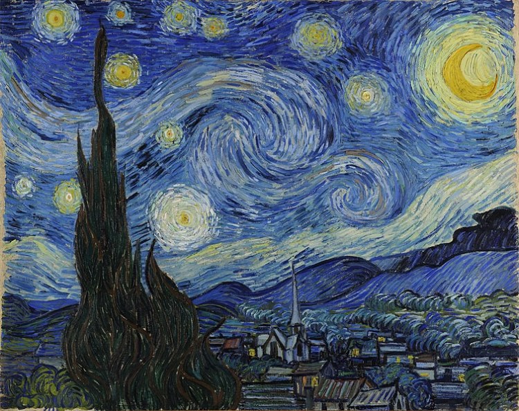
Neural style transfer is an optimization technique used to take two images- an image and a style reference image (such as an artwork by a famous painter)-and blend them together so the output image looks like the content image, but “painted” in the style of the style reference image.
Big Data Jobs
This is implemented by optimizing the output image to match the content statistics of the content image and the style statistics of the style reference image. These statistics are extracted from the images using a convolutional network.
# Create a simple function to display an image:
def imshow(image, title=None):
    if len(image.shape) > 3:
    image = tf.squeeze(image, axis=0)

plt.imshow(image)
if title:
    plt.title(title)
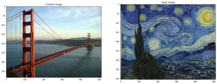
# Download images and choose a style image and a content image: content_path = tf.keras.utils.get_file('Golden_Gate.jpg', 'https://upload.wikimedia.org/wikipedia/commons/0/0c/GoldenGateBridge-001.jpg')
Let’s confirm that we have downloaded and loaded correctly the images.
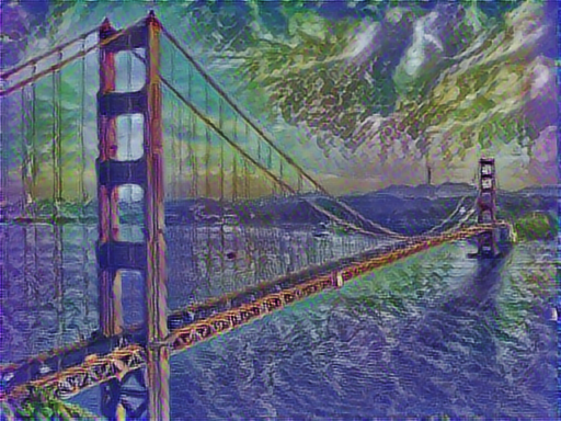
# Use the TensorFlow Hub
import tensorflow_hub as hub
hub_module = hub.load('https://tfhub.dev/google/magenta/arbitrary-image-stylization-v1-256/1')
stylized_image = hub_module(tf.constant(content_image),tf.constant(style_image))[0]
tensor_to_image(stylized_image)
Discussion
That was a practical example of how you can easily apply Neural Style Transfer and to be somehow a “digital artist” :-). Note that modern approaches train a model to generate the stylized image directly (similar to cyclegan).
Understanding the evaluation metrics for recommender systems
In this post, we will be discussing evaluation metrics for recommender systems and try to clearly explain them. But before that let’s understand the recommender system in short.
A recommender system is an algorithm that provides recommendations to users based on their historical preferences/ tastes. Nowadays, recommendation systems are used abundantly in our everyday interactions with apps and sites. For example, Amazon is using them to recommend products, Spotify to recommend music, YouTube to recommend videos, Netflix to recommend movies.
The quality of the recommendations is based on how relevant they are to the users and also they need to be interesting. When the recommendations are too obvious, they are not useful and mundane. For the relevancy of recommendation, we use metrics like recall and precision. For the latter (serendipity) metrics like diversity, coverage, serendipity, and novelty are used. We will be exploring the relevancy metrics here, for the metrics of serendipity, please have a look at this post: Recommender Systems — It’s Not All About the Accuracy.
Big Data Jobs
Let’s say that there are some users and some items, like movies, songs, or products. Each user might be interested in some items. We recommend a few items (the number is k) for each user. Now, how will you find whether our recommendations to every user were efficient?
In a classification problem, we usually use the precision and recall evaluation metrics. Similarly, for recommender systems, we use a mix of precision and recall — Mean Average Precision (MAP) metric, specifically MAP@k, where k recommendations are provided.
Let’s explain MAP, so the M is just an average (mean) of APs, average precision, of all users. In other words, we take the mean for average precision, hence Mean Average Precision. If we have 1000 users, we sum APs for each user and divide the sum by 1000. This is the MAP.
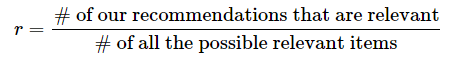
So now, what is average precision? Before that let’s understand recall (r)and precision (P).
PrecisionRecall
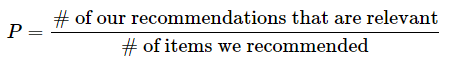
There is usually an inverse relationship between recall and precision. Precision is concerned about how many recommendations are relevant among the providedrecommendations. Recall is concerned about how many recommendations are provided among all the relevant recommendations.
Let’s understand the definitions of recall@k and precision@k, assume we are providing 5 recommendations in this order — 1 0 1 0 1, where 1 represents relevant and 0 irrelevant. So the precision@k at different values of k will be precision@3 is 2/3, precision@4 is 2/4, and precision@5 is 3/5. The recall@k would be, recall@3 is 2/3, recall@4 is 2/3, and recall@5 is 3/3.
So we don’t really need to understand average precision (AP). But we need to know this:
we can recommend at most k items for each user
it is better to submit all k recommendations because we are not penalized for bad guesses
order matters, so it’s better to submit more certain recommendations first, followed by recommendations we are less sure about
So basically we select k best recommendations (in order) and that’s it.
Here’s another way to understand average precision. You can think of it this way: you type something in Google and it shows you 10 results. It’s probably best if all of them were relevant. But, if only some are relevant, say five of them, then it’s much better if the relevant ones are shown first. It would be bad if the first five were irrelevant and good ones only started from sixth, wouldn’t it? AP score reflects this. They should have named it ‘order-matters recall’ instead of average precision.
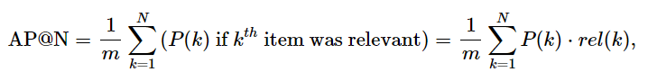
But if you persist, let’s dive down into the math. If we are asked to recommend N items and the number of relevant items in the full space of items is m, then:
Average Precision
where P(k) is the precision value at the kth recommendation, rel(k) is just an indicator that says whether that kth recommendation was relevant (rel(k)=1) or not (rel(k)=0).
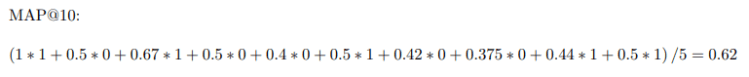
Consider, there are 5 relevant recommendations (m), we are making 10 recommendations (N) as follows — 1 0 1 0 0 1 0 0 1 1. Let’s calculate the mean average precision here.
Compare the math with the above formula and you will understand the intuition. Now to proof that MAP takes care of the order, as we mentioned earlier, let’s provide another set of recommendation — 1 1 1 0 1 1 0 0 0 (here we are making relevant recommendations first).
To summarize, MAP computes the mean of the Average Precision (AP) over all the users for a recommendation system. The AP is a measure that takes in a ranked list of the k recommendations and compares it to a list of relevant recommendations for the user. AP rewards you for having a lot of relevant recommendations in the list, and rewards you for putting the most relevant recommendations at the top.
Language-guided navigation is a widely studied field and a very complex one. Indeed, it may seem simple for a human to just walk through a house to get to your coffee that you left on your nightstand to the left of your bed. But it is a whole other story for an agent, which is an autonomous AI-driven system using deep learning to perform tasks.
Indeed, current approaches try to understand how to move in a 3D environment in order to let the agent freely move like a human. This new approach I will be covering in this article changes that by letting the agent only executing low-level actions in order to follow language navigation directions, such as “Enter the house, walk to your bedroom, go in front of the nightstand to the left of your bed.”
They’ve achieved this by using only four actions; “Turn-left”, “Turn-right”, “move forward for 0.25 m”, “Stop”. This allowed the researchers to lift a number of assumptions that prior work were using, such as the need to know exactly where your agent is at all time.
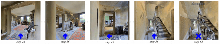
Using this technique makes the trajectories significantly longer, using an average of 55.88 steps rather than 4 to 6 steps from current approaches. But again, these steps are much smaller and make the agent much more precise and “human-like.”
Let’s see how they achieved such thing and some amazing examples. Feel free to read the paper and check out their code, which are both linked at the end of this article.
As the name says, they developed a language-guided navigation task for 3D environments where the agents follow language navigation directions given by a user in order to realistically move in the environment.
In short, the agent is given first-person vision, which they call Egocentric, and a human-generated instruction, such as this example; “Leave the bedroom and enter the kitchen. Walk forward and take a left at the couch. Stop in front of the window.” Then, using this input alone, the agent must take a series of simple control actions like “move forward for 0.25 m”, “turn left for 15 degrees”, to navigate to the goal. Using such simple actions, VLN-CE lifts assumptions of the original VLN task and aims to bring simulated agents closer to reality. Just to give a comparison, current state-of-the-art approaches move between panoramas and cover 2.25 meters on average including avoiding obstacles for a single action.
Big Data Jobs
The 2-model method
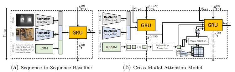
They developped two different models in order to achieve such task. The first one (a) is a simple sequence-to-sequence baseline. The second one (b) is a more powerful cross-modal attentional model, which we can both see in this picture.
This first model takes a visual representation of the observation, containing depth and RGB features, and instructions for each time step. Then, using this information and the instructions given by the user, it predicts a series of action to take, denoted as “at” in this image.
The RGB frames and depths are respectively encoded using two ResNets-50 architectures, one pre-trained on ImageNet and the other one trained to perform point-goal navigation.
Then, it uses an LSTM to encode the instructions from the user. LSTM is the short for Long short-term memory, which is a recurrent neural network architecture widely used in natural language processing applications due to its memory capabilities allowing it to use previous words information as well.
These actions, a, are then fed into the second model. The goal of this second model is to compensate for the lack of visual reasoning in the first model, which is super important for this kind of navigation application.
For example, you need a good spatial visual reasoning in order to understand an instruction such as “to the left of the table.” Your agent needs to know that it first needs to know where’s the table, and then, go to the left of that table.
[Photo by Romain Vignes on Unsplash]
Which is done using attention. Attention is basically based on a common intuition that we “attend to” a certain part when processing a large amount of information, like the pixels of an image. More specifically, it is done using two recurrent networks, as you can see in the image, one tracking observations using the same RGB and depths input as the first model.
While the other network’s role is to make decisions based on the user’s fed instructions and visual features.
This time, the user’s instructions are encoded using a bidirectional LSTM. Then, they compute a list of simple instructions which is used to extract both visual and depth features.
Following that, the second recurrent network uses a concatenation of all the features discussed including an action encoding as inputs and predicts a final action.
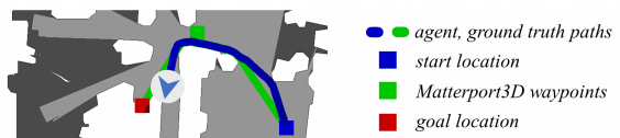
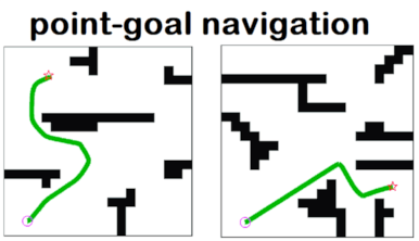
To train such task, they used a total of 4475 trajectories split from the train and validation split. For each of those trajectories, they provided multiple language instructions and an annotated “shortest path ground truth via low-level actions” as seen in this image.
At first, it looks like it needs a lot more details and time to achieve such task. Shown in this picture below, where (a) being the current approaches, using real-time localization of the agent, and (b) being the covered approach with low-level actions.
But when we compare it to the traditional panoramic view with perfect location instead of having no position given and using only low-level actions it is clear that it needs way less computation time in order to succeed, just as you can see in the amount of information given for each approaches in the picture above.
Results
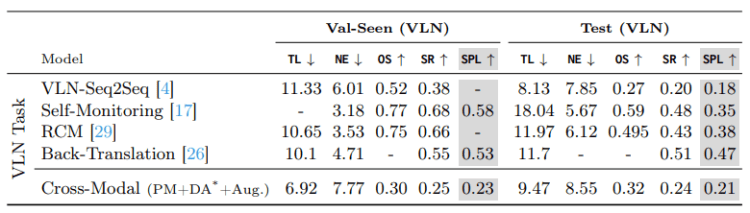
This is a comparison on the VLN validation/test datasets between this and the current state-of-the-art approaches.
From these quantitative results, we can clearly see that using this cross-modal approach with multiple low-level actions in a continuous environment outperforms the nav-graph navigation approaches in every way. It is hard to visualize such results from a theoretical comparison basis, so here are some impressive examples using this new technique:
Watch the video to see more examples of this new technique:
I invite you to check out the public release version of the code on their GitHub. Of course, this was just an introduction to the paper. Both are linked below for more information.
Algorithms for text analytics must model how language works to incorporate meaning in language—and so do the people deploying these algorithms. Bender & Lascarides 2019 is an accessible overview of what the field of linguistics can teach NLP about how meaning is encoded in human languages.
Amazon’s Machine Learning University is making its online courses available to the public, and this time we look at its Accelerated Computer Vision offering.
Computer vision is the simply the process of perceiving the images and videos available in the digital formats.
In Machine Learning (ML) and AI — Computer vision is used to train the model recognize certain patterns and store the data into their artificial memory to utilize the same for predicting the results in real-life use
The application of computer vision in artificial intelligence is becoming unlimited and now expanded into emerging fields like automotive, healthcare, retail, robotics, agriculture, autonomous flaying like drones and manufacturing etc…
Machine Learning Jobs
So here in this blog by enabling the power of deep learning , we will show you that how we can solve one of the problem of computer vision called ‘ Image Segmentation ’
Image Segmentation is a task of computer vision in which we partitioning images into different segments.
yes, sounds like Object detection , but no it different task than object detection …. Because Object Detection methods helps us draw bounding boxes around certain entities/Objects in Given Image ,
But on other side Image segmentation lets us achieve more detailed understanding of imagery than image classification or object detection.
in Simple words , in Image Segmentation we basically assign/classify each pixel to a particular class.
Semantic segmentation — classifies all the pixels of an image into meaningful classes of objects. These classes are “semantically interpretable” and correspond to real-world categories. For instance, you could isolate all the pixels associated with a cat and color them green. This is also known as dense prediction because it predicts the meaning of each pixel.
Instance segmentation — identifies each instance of each object in an image. It differs from semantic segmentation in that it doesn’t categorize every pixel. If there are three cars in an image, semantic segmentation classifies all the cars as one instance, while instance segmentation identifies each individual car.
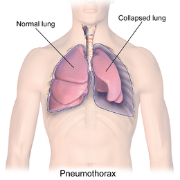
This Problem basically from the Healthcare domain. imagine suddenly gasping for air, helplessly breathless for no apparent reason. Could it be a collapsed lung? In the future, we are going to predict this answer.
Pneumothorax can be caused by chest injury, damage from underlying lung disease, or most horrifying — it may occur for no obvious reason at all. On some occasions, a collapsed lung can be a life-threatening event.
Pneumothorax is usually diagnosed by a radiologist on a chest x-ray images ,but sometimes it could be difficult to confirm.
Pneumothorax is visually diagnosed by radiologist, and even for a professional with years of experience; it is difficult to confirm.
So Our Goal is to Detect and Segment those Pneumothorax affected area with a help of Semantic Segmentation methods,so that we can help the radiologist by giving the results with higher precision.
Solution:
An AI algorithm to detect Pneumothorax would be useful to Solve this problem,
we will try to solve this problem in two Phase:
1 Pneumothorax Classification:
2 Pneumothorax Segmentation
So, in first phase we will develope a classification model to classify Pneumothorax and in Second Phase we will build a model for segmentaiton task on given image
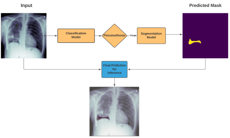
How prediction pipeline will work?
if Classification model detects the Pneumothorax in input X-Ray image then our Prediction Pipeline will pass that X-Ray image to Segmentation Model to segment the Pneumothorax in That X-ray image so that Radiology Expert can easily Analyze and Diagnose this Problem
This is How our Final Pipeline will Work
4. Dataset :
Before Going to Understand the Classification & Segmentation Architectures, let’s Have a glance at Dataset,
here we are using dataset which has been modified from the kaggle competition’s dataset.
so that we can easily get our input and target mask in (.png format).
Before start the Explaination Deep Learning Architecture, i assume that you have guys have a good Understanding of Basic Convolutional Operations like,
Conv2d, UpSampling , Dense Layers, Upconv2d Layer, Conv2dTranspose Layer , Softmax, Relu, BatchNormalisation all Basic stuff of Deep Learning with keras and most important Residual Block (ResNet & DenseNet).
5. Classification & Segmentation Architecture:
As you know that we have divided this problem into 2 part , So let’s have a look at part-1,
Part 1 : Pneumothorax Classification:
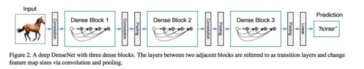
Basically here to solve this Classification problem , we have used DenseNet121 Architecture.
DenseNet is One of the new Architecute for image classification & Object Recognition , it is quite similar to ResNet Architecture with some fundamental differences, ResNet uses an additive method (+) that merges the previous layer (identity) with the future layer, whereas DenseNet concatenates (.) the output of the previous layer with the future layer.
here for our problem i used the DensNet-121 architecture Using this package,
from tensorflow.keras.applications.densenet import DenseNet121
But there is one more important thing that i have used to get state of the art results is, for Transfer Learning instead of using pre-trained weights of imagenet , i have used the weights of ChestXpert — DenseNet , because this ChestXpert model was trained on Medical X-Ray images to classify around 14 Disease which was related to Lungs.
and Pneumothorax was one of them so i directly loaded the weights of ChestXpert model for our DenseNet-121 but only for all convolutional blocks , and for dense layer i have initialized the weights using keras..
Below is the keras code to implement the above model,
from tensorflow.keras.applications.densenet import DenseNet121
from tensorflow.keras.layers import Dense, Input
from tensorflow.keras.models import Model, load_model
  #create the base pre-trained model
  base_model = DenseNet121(include_top=False,
                           input_tensor=img_input,
                           input_shape=input_shape,
                           weights=base_weights,
                           pooling='avg')
  x = base_model.output

  # add a logistic layer -- let's say we have 14 classes
  predictions = Dense(14,activation='sigmoid',name='predictions')(x)
  # this is the model we will use
  model = Model(inputs=img_input,
                outputs=predictions,)
tf.random.set_seed(1234)
base, model = get_chexnet_model()
x = Dense(1024, activation='relu', kernel_initializer='he_normal')(model.layers[-2].output)
x = Dense(2, activation='softmax', kernel_initializer='he_normal')(x)
and we achieved 90%Accuracy on trainset and 87% Accuracy on validation set….
So now after completing the part 1 ,Let’s have a look at Part -2
Part 2: Pneumothorax Segmentation:
Now we will discuss most important part of this blog ,
For this task we have implemented the Architecture called ” UNet++ : nested UNet architecture” , it is the advanced or can say extended version of UNet.
to Understand this architecture must have basic idea about how UNet work for Semantic segmentation , you can read this to understand the UNet Architecture.
So i hope now you will have a better understandings of UNet.
UNet++ : Nested UNet architecture for Medical Image Segmentaion:
So as you can see in this diagram so we will find some similarites between UNet and UNet++
Because Like Unet , UNet++ also follows the same encoder-decoder approch to generate the semantic segmentation
But here i have mentioned some points which differs UNet++ from UNet:
Convolution layer on skip pathways which bridges the semantic gap between encoder-decoder
Dense skip connections at skip pahways which improves the Gradient flow and prevents from gradient vanishing problem
Deep Supervision which improves the model pruning
that’s it , But if you want to go more deeper to understand How this things work in UNet++ then you from here you will get the better idea
Below keras code will help you to define above model (UNet++):
def convolution_block(x,filters,\
                      size,strides(1,1),\
                      padding='same',activation=True):
 x = BatchNormalization()(x)
 if activation == True:
  x = LeakyReLU(alpha=0.1)(x)
 return x
def residual_block(blockInput, num_filters=16):
  x = LeakyReLU(alpha=0.1)(blockInput)
  x = BatchNormalization()(x)
  blockInput = BatchNormalization()(blockInput)
  x = convolution_block(x, num_filters, (3,3) )
  x = convolution_block(x, num_filters, (3,3), activation=False)
  x = Add()([x, blockInput])
  return x
model = Model(input, output_layer) model.name = 'u-xception' return model
tf.keras.backend.clear_session()
img_size = 256
model = UEfficientNet(input_shape=(img_size,img_size,3),dropout_rate=0.3)
Training:
To train this model , I used
Dice_Loss:
Generally for image segementation task , combination of binary cross_entropy and Dice_loss is being used immensely ,
because as we all know only binary cross entropy is not good option while you will having an imbalanced dataset , but here this Dice_loss works excellenty in those scenario ,
so our final loss will be
loss function = Binary_crossentropy + Dice_Loss, where N=Batch_size
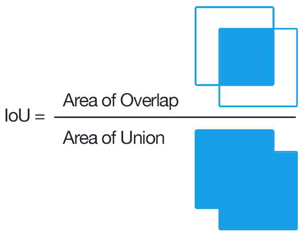
IoU_Score (Intersection over Union):
so we have talked about loss, but what about Evaluation Metrics, should we use Accuracy ???
so Answer is No, for Image Segmenation or Object Localization task IoU_score is being Used extensively ,
Basically Accuracy function will also take those region/pixels which is not part of that object in specific image , specially for medical image segmentation task in which targeted mask contains very less amount of pixel , so in that case accuracy will always be high without taking care about location of the affected region by disease,
after looking at this diagram , you would have get the idea about how IoU Score works ,
It comes in handy when you’re measuring how close an annotation or test output lines up with the ground truth. As a ratio of the areas of intersection and union, it works on annotations of all shapes and size.
What’s cool is how IOU can be used with F1 scores to measure the accuracy of object detection tasks with multiple annotations per image
so after set the loss and evaluation matrice , we train this model using adam as an optimiser for 40 epochs,
so after 40 epochs of training we were able to get 0.73 IoU_Score and 0.71 val_IoU_Score.
7. Inference Pipeline:-
So as I mentioned in earlier in Inference pipeline’s Diagram ,
we will only predict the segmentation mask for input Chest X-Ray image if our Classifier will detects any Pneumothorax in that X-ray Image, otherwise there is no mean to predict the segmentation mask for that
here i am showing some predictions of our segmentation model…
Green: Groundtruth mask Red: Predicted mask
Here, Green Pixels Represents the Groundtruth (Actual Mask) & Red Pixels Represents the Predicted Mask.
we we have developed the complete Class called Pipeline for final production pipeline.
if pre_cls==1: img_seg = self.segmentation.predict(tf.expand_dims(image, axis=0), steps=1) plt.imshow(img_seg[0,:,:,0], cmap='Reds', alpha = 0.4) plt.title("Pneumothorax is Detected.........")
    else:
      plt.title("Pneumothorax is not Detected.........")
    plt.show()
So our pipeline will segment the predicted mask by presenting it in red region , which will show the location of Pneumothorax in given input X-Ray image of Patient
8. Conclusion :-
i really appreciate you for giving time to read this blog
so please clap it if you like and learn new things from this blog , because it will encourage me to share more knowledge and informations related to Deep Learning through my blogs.