365 Data Science is an online educational career website that offers the incredible opportunity to find your way into the data science world no matter your previous knowledge and experience.
In this article I would like to focus on how companies can start their data-centric strategies and how to achieve success in their data transformation journeys. Have tried to share my thoughts why companies have to consider data at its epitome for their growth, for being competitive, for being smarter, innovative and be prepared for any unforeseen market surprises.
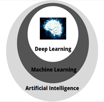
Deep learning is a subset of machine learning, which in turn is a subset of Artificial intelligence.
Artificial intelligence involves traditional methods to learn from data, whereas machine learning involves teaching the computer to recognize pattern from the data. Deep learning is a machine learning technique that learns features directly from the data by using an architecture called “neural networks”.
Why deep learning?
No matter how complex the traditional machine learning algorithm gets, it will still be machine-like and can perform only designated tasks. They are very domain specific. Hence, to overcome these disadvantages we go for more advanced branch of machine learning which is deep learning. Moreover, Deep learning provides us with the advantage of learning by itself from raw data!
Jobs in AI
Many of the deep learning algorithms already existed for many years, but it is now, that they are gaining popularity. In general, three technical forces are driving advances in machine learning: advance hardware and great computational power, abundance of data and availability of open source software like TensorFlow and PyTorch etc.
Neural Networks
Neural Networks form the base of deep learning and the fundamental building block of the neural network is a neuron. The neural networks take data as their input, train themselves using the data and present useful predictions as their outputs.
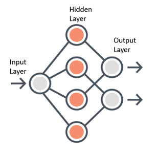
Any neural network is made up of three essential components — Input layer, Several hidden layers and an output layer.
Sample Neural Network
Learning of a Neural Network
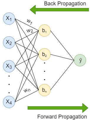
Learning process of a Neural Network includes two parts — Forward propagation and Back propagation.
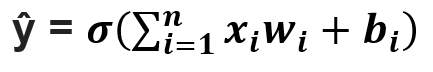
Forward propagation is the flow of information from the input layer to the output layer. Input layer consists of several neurons which are connected to the next layer through channels, which are assigned numerical values know as weights(wᵢ) (At the beginning of the process the weights are randomly assigned and later updated). The data fed into the input layer(xᵢ) is multiplied by these weights and then fed into the next layer. All the neurons in the hidden layer are associated with a value know was bias(bᵢ) which is then added to the input sum. This weighted sum is then passed through the non- linear function called the activation function(σ). This function decides whether a particular neuron can contribute to the next layer. Finally the output layer gives the probability, the neuron with the highest probability is finaloutput(ŷ). This process is represented in mathematical form as:
(Don’t be afraid of the big equation, it is just the mathematical representation of the above explanation, read the explanation along with the equation again and you are good to go!)
Back propagation is same as the forward propagation but in reverse direction. The information is passed from the output layer to the input layer. After the last layer gives a prediction, it is evaluated by a loss function. The loss function helps quantify the deviation from the expected output, meaning it gives a value that depicts the difference between the predicted output and the actual output. This information is sent back to the hidden layer to adjust the weights and bias to get a more accurate prediction. The weights and bias are updated using the gradient descent algorithm(optimizer).
Note: Weights and Biases are known as theModel parameterswhereas the learning rate is known as theModel Hyperparameter.
Important Terminologies
Let’s see some important terms quickly:
Weights: Basically it tells us how important a channel(link between the two neurons) is. The higher the value the more important it is.
Bias: It allows to shift the activation function to the right or left (as adding a scalar value to a function shifts the graph to the right or left)
Activation function: Introduces non- linearity in the network and also decides whether a neuron can contribute to the next layer. Step function, Linear function, Sigmoid function etc. are some examples of the activation function.
Loss function: Loss function are the mathematical ways of measuring how wrong the predictions made by the neural network are. Depending on the project you are working on you can use different loss functions like squared error, binary cross entropy, multi- class cross- entropy etc.
Optimizer: Update the weights and bias in response to the output of the loss function. The loss function acts like a guide to the optimizer which tells whether it moves in the right or wrong direction. The goal of the optimizer is to minimize the loss function. The most popular optimizer is gradient descent.
Learning rate: Learning rate ensures that changes made to the weights are at the right pace. Taking too large steps or too small steps can mean that the algorithm will never find optimum values for the weights.
Epochs: One epoch is when the entire dataset is passed forward and backward through the neural network only once. Generally, we use more than one epoch. Passing the dataset multiple times to the network helps the model to generalize better. But too many epochs may cause the problem of overfitting(model makes prediction specific to the dataset rather than making more general predictions).
Batches, Batch sizes: Datasets includes millions of examples, passing the entire dataset at once becomes extremely difficult. Hence, we divide the dataset in smaller chunks or batches and then feed it to the neural network. Number of examples in one batch is the batch size.
Iterations: Size of the dataset divided by batch size gives us the number of iterations. E.g. If you have a dataset of 39,000 training examples and you divide the dataset into batches of 600, then you will have 39,000/600 = 65 iterations to complete one epoch.
Note:There is no right combination of number of hidden layers, activation function, number of epochs etc. which will give maximum accuracy to your model. You will have toexperimentand find out what suits best for your project!
Regularization
One of the main goal of deep learning is to build a model that will perform well not only on training data but also on new inputs. Overfitting is a situation when the model performs exceptionally well on the training data but not on testing data. It probably learns “too much” from the training data. Regularization is a technique to avoid overfitting. Some regularization technique are — Dropout, Augmentation, Early Stopping.
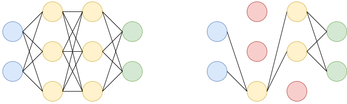
Dropout: Let’s say we have a neural network with two hidden layers. During each iteration, dropout randomly selects some nodes and removes them along with their connections as shown in the diagram(red nodes are dropped).
So each iteration has different sets of nodes which result in different sets of output which help in better generalizing the model as it captures more random features.
Augmentation: Another cause of overfitting is having too few examples to learn from. Augmentation refers to creating more training data from existing data by applying various transformations. This helps the model to expose to more aspects of the data and generalize better.
Early Stopping: When training over sufficient data, we often observe that the training error decreases with time but the error begins to rise again. Thus we can obtain a better model if we stop training when an increase in error is observed, this is known as early stopping.
Neural Network Architecture
The three most common type of neural networks are:
Fully connected feed forward neural network
Fully connected indicates that each neuron in preceding layer is connected to every other neuron in the following layer, in only forward direction(no backward connections or loops).
Recurrent Neural Network(RNN)
Fully connected or plain neural networks cannot handle sequential data. Processing of sequential data, may require information from the earlier stage of processing and plain neural networks don’t share parameters across time. RNN has the ability to look for a given feature everywhere in the sequence, rather than in just a certain area. RNN uses feedback loop in the hidden layer.
Convolutional Neural Network(CNN)
CNN is a deep neural network architecture which is used specifically for tasks like image classification, processing audios, videos etc. Hidden layers of CNN include convolutional layer, pooling layer, fully connected layer, normalization layer instead of traditional activation functions.
Create a deep learning model
There are five fundamental steps involved in every deep learning project. They can be extended to many other steps, but at the very core there are five.
10 Ways How AI can Transform the Education Industry
The advent of artificial intelligence in the education industry has benefited both students and teachers. The merger of this technology with today’s education system is revolutionizing the way students understand a concept and learn new things.
Besides this, the technology has also changed the way teachers used to teach; they can now use real-life examples to make their students learn better and quicker. AI, if used to its full potential, can take the education world by storm. Didn’t believe us? Let’s dig deeper to know the ten amazing roles of artificial intelligence in this industry:
Ten uses of artificial intelligence in education
1. Personalized learning
2. AI-powered assistants
3. Smart content
4. Automating grading and other activities
5. AI tutors
6. Improved teaching and studying
7. Better engagement
8. Crafting courses
9. Monitoring students’ performance
10. AI-based programs to get valuable feedback
Let’s read them in detail:
Personalized learning
AI can help teachers to offer customized learning to help students learn as per their capability. Some of the renowned education platforms, such as Carnegie Learning, are already using artificial intelligence to offer personalized courses. The technology can also help in providing specialized instructions created particularly for an individual.
Jobs in AI
AI-powered assistants
With the help of AI-powered assistants, students can access learning materials without even contacting a teacher. To take as an example, Arizona State University uses Alexa to help students with daily campus requirements. Alexa can provide answers to student’s queries and help them to find other information.
Smart content
An AI-based program can efficiently handle and analyze big data (in this case, various learning materials available on the web) to fetch the relevant information for students. Companies like Netex Learning is helping students with their personalized cloud platforms that further offer conferences, virtual training, and other educational services.
Automating grading and other activities
The process of grading homework and assignments eats up a lot of time that could be used for preparing the class or teaching students. While it is evident that AI cannot completely replace a teacher, but it can become a helping hand to assess and give grades for the tests that include multiple-choice questions or fill in the blanks.
Having an AI-based tutor is a fantasy yet, but the way this technology is improving, this could soon be a reality. Some of the AI-based programs, acting as a tutor, are already there in the industry to help students to learn Basic English, mathematics, and other subjects.
Improved teaching and studying
Using different AI-powered software, teachers can help students to understand a concept better. They can use real-life examples and show them to the students to tell how things actually work.
Better engagement
There are many AI-based platforms where students can discuss the problems they are facing while learning a particular subject or understanding a topic. These platforms are a suitable way to connect with other peers to share knowledge, which increases the engagement level.
Crafting courses
AI-based software can also help teachers to fill the gap between the educational materials and their lectures. Such software can aid them to craft customized courses and the ways to improve them to teach better. For instance- Coursera, a well-renowned e-courses provider, is already using this technology to alert teachers whenever a large number of students submit an incorrect answer to a question.
Monitoring students’ performance
Using AI-based teaching software, teachers can keep track of student’s performance and know how much they have improved or where they require improvement. In this way, they can pay attention to each student’s requirements.
AI-based programs to get valuable feedback
Schools, colleges, and other educational institutions that are currently offering online programs are using AI-based software to track the progress of students and to alert teachers about the performance of a student.
Use Cases of AI in Education
· Brainly
Brainly is a social platform that helps students to cooperate and discuss the problems they find in doing their homework. This largest peer-to-peer learning community for students, parents and teachers uses artificial intelligence and machine learning to offer personalized materials and identify inappropriate content.
· ThinkerMath
The main aim of this AI-based solution is to aid small kids to learn Math. It offers personalized learning as per the knowledge of every individual student. To improve students’ engagement, ThinkerMath offers many games and rewards.
· CTI
Harnessing the potential of artificial intelligence, CTI develops smart content by analyzing textbooks and other learning material to bring out important information for users.
Why choose Quytech to AI-based education app development?
Quytech is backed by a team of experienced and skilled AI developers with considerable experience of working on artificial intelligence, machine learning, natural language processing, computer vision, and other technologies. Besides this, there are many other reasons for choosing our company to develop an AI-enabled education app:
· On-time delivery- We guarantee to design, develop, and deploy your project within the specified period.
· Post-launch support and maintenance– To integrate new technologies & features and to keep your app bug-free, we offer post-launch support and maintenance services.
· Flexible plans- You can either choose our app development services or hire our AI app developers on a monthly or hourly basis.
· Expertise in the domain- We have successfully developed and deployed many AI-based applications to renowned schools, universities, and colleges worldwide.
To begin developing your AI-powered education app, or to integrate this technology in your existing education app, contact us right away. We are just a call away!
Final Words
It is unarguably true that artificial intelligence has transformed the standard way of teaching and getting an education. That’s why colleges, schools, and universities are investing heavily to make AI as a vital part of their education system. The technology can automate activities like grading, upgrade the education software, help in improvisation of various courses, teach pupils, and provide many other advantages. So, if you are looking out for building an AI-based education app or integrate AI in your education mobile application, then connect to a reliable mobile app development company now.
With more advancements in AI, it might be time to replace the age-old Turing Test with something better to determine if a machine is thinking. Specifically, a more modern approach might include standard questions designed to probe various facets of intelligence, and comparing the computer to a spectrum of human respondents of different ages, sexes, backgrounds, and abilities.
Inspired by Judea Pearl’s do-calculus for causal inference, the open source framework provides a programmatic interface for popular causal inference methods.
With ML models serving real people, misclassified cases (which are a natural consequence of using ML) are affecting peoples’ lives and sometimes treating them very unfairly. It makes the ability to explain your models’ predictions a requirement rather than just a nice to have.
Welcome back! In my previous post I wrote an EDA (Exploratory Data Analysis) on Titanic Survival dataset. Check it out now if you haven’t already. Anyway, in this article I would like to be more focusing on how to create a machine learning model which is able to predict whether a Titanic passenger survived based on their attributes i.e. gender, title, age and many more.
Before going any further, I also want you to know that the project I do here is inspired by this article: https://towardsdatascience.com/kaggle-titanic-machine-learning-model-top-7-fa4523b7c40. I do implement several feature engineering techniques explained in that article with several modifications for the sake of simplicity. Now let’s do this 🙂
Note: full code available at the end of this article.
As always, the very first thing I do is importing all required modules and loading the dataset.
import pandas as pd
import numpy as np
import matplotlib.pyplot as plt
import seaborn as sns; sns.set()
from sklearn.linear_model import LogisticRegression
from sklearn.model_selection import train_test_split
from sklearn.metrics import confusion_matrix
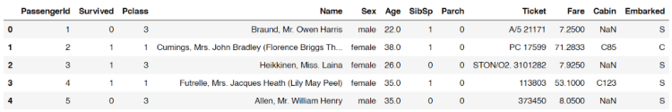
df = pd.read_csv('train.csv')
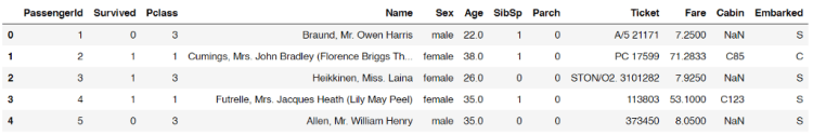
The first 5 data in Titanic dataset.Big Data Jobs
Feature engineering 1: SibSp & Parch
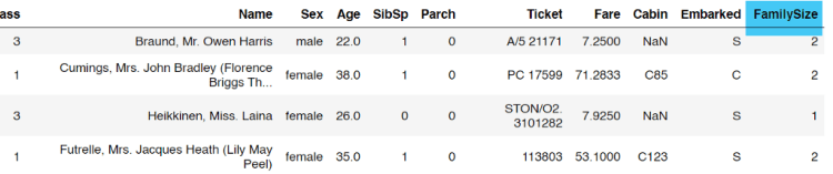
Now let’s start the feature engineering stuff from the SibSp and Parch columns. According to the dataset details (which you can access it from this link), the two columns represent the number of siblings/spouses and the number of parents/children abroad the Titanic respectively. The idea here is to create a new column called FamilySize in which the value is taken from the two columns I mentioned earlier. This action is taken based on the assumption that larger family size may have greater opportunity to get survived as they can stay intact with each other better than those who travel alone. Below is the code to do that.
And here’s how our new data frame df looks like. We can see here that the FamilySize column appears as expected.
Adding FamilySize column.
Feature engineering 2: Embarked
According to the EDA explained in my previous article, there are 2 missing values in Embarked column. Since it’s not a significant number, we are just gonna eliminate them:
df = df.dropna(subset=['Embarked'])
The argument subset indicates that the code will drop rows with NaN values in Embarked column only.
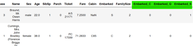
Next, if we take the unique values of this column, we will find that there are 3 possible values, namely C, Q and S (which stands for Cherbourg, Queenstown and Southampton). Here I decided to convert this column values into something like one-hot representation since any machine learning algorithm will never work with non-numerical data. To do that, we can use get_dummies() function coming with Pandas module.
The first line of the code above shows that the one-hot-encoded values are stored in embarked_one_hot variable. Then, the variable is concatenated with our original data frame df.
One-hot representation of Embarked column is concatenated to the original data frame.
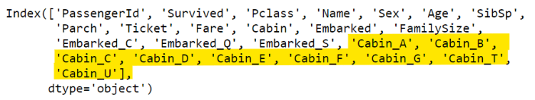
Feature engineering 3: Cabin
In my previous post (EDA of this Titanic dataset), I found that the values of Cabin column contains plenty of missing values. Thus, I decided to fill that out with U, which stands for “Unknown”. It can simply be achieved using fillna() method.
df['Cabin'] = df['Cabin'].fillna('U')
Next, I also found that the values of that column are a letter followed with several numbers (also explained in the previous post). What I wanna do now is to extract all those initial characters. My approach here is to employ lambda function like this:
df[‘Cabin’] = df[‘Cabin’].apply(lambda x: x[0])
Now that all values of Cabin column have been updated to only a single letter. The next step to do is to convert the value of this column into one-hot format. To do that, I will use the exact same method as what we have done to Embarked column.
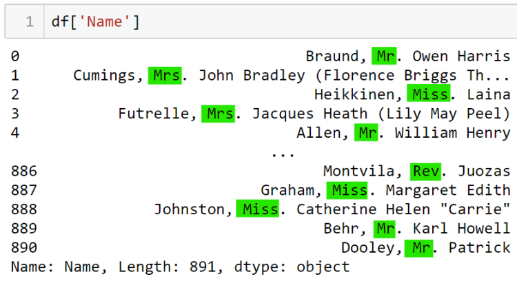
You probably might be thinking at the first place that we don’t even need to take into account the values of Name column as it only holds the name of a person. Theoretically, name will never affect the survival chance of a person. And yes, I do agree with that. However, if we pay closer attention to its contents, we are going to find something interesting: title.
We are going to take all these titles.
Those titles may be a good feature to consider whether this person is survived or not. Therefore, we are going to take these titles using get_title() function that we declare manually by ourselves.
Now as the function has been declared, we can just apply that function to Name column and store the result to a new column Title.
df['Title'] = df['Name'].apply(get_title)
If you want, you can also check the unique values stored in Title column using df[‘Title’].unique() command. The output is going to look something like this:
Similar to the Cabin column, we are going to convert the values of Title into one-hot representation because up to this stage its values are still in form of categorical data. Below is my approach to do so.
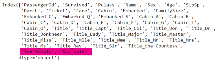
Well, I guess there’s no much thing to say here. We know that there are only two values in in Sex column, namely female and male, which we know that this is also a categorical data. Therefore, we can simply use pd.get_dummies() function again to convert the values of this column into one-hot format.
We can clearly see here that two new sex columns have been successfully created.
Feature engineering 6: Age
If I were to say, this Age feature engineering is the most tricky part — well, at least for me. According to my previous article which talks about EDA on this Titanic dataset, we found that 177 out of 889 passengers’ age are missing. Therefore, we need to fill this with a number. However, in this case we will not just directly fill those NaNs with the median or mean of all existing age numbers. Instead, I wanna group all passengers data by its Title first, and then compute the median of each title group before eventually use these medians to fill the missing values. Here’s the first thing to do:
After running the code above, we are going to obtain the median of each Title.
Title
Capt            70.0
Col             58.0
Don             40.0
Dr              46.5
Jonkheer        38.0
Lady            48.0
Major           48.5
Master           3.5
Miss            21.0
Mlle            24.0
Mme             24.0
Mr              30.0
Mrs             35.0
Ms              28.0
Rev             46.5
Sir             49.0
the Countess    33.0
Name: Age, dtype: float64
Next, we need to create a function fill_age() which accepts a single value as its parameter. This x parameter basically just represents every row in our data frame.
def fill_age(x):
    for index, age in zip(age_median.index, age_median.values):
        if x['Title'] == index:
            return age
Now it’s time to apply this fill_age() function. However though, we need to be careful since essentially what we need to do is to replace only the missing Age, not the entire values in Age column. Therefore, I define a lambda function inside of apply() method. What’s actually done by the lambda function itself is that we are going to apply the fill_age() function only when the corresponding age is missing. Otherwise, if the age value already exists, then we will just use its existing value. Below is how to do it:
df['Age'] = df.apply(lambda x: fill_age(x) if np.isnan(x['Age']) else x['Age'], axis=1)
Now if we try to run df.isnull().sum(), we will see that our data frame df no longer contains missing value. But remember that some of our columns are still using categorical type. We can check it by running df.dtypes.
Now, the very last step in feature engineering part is to normalize all values. In this project I decided to use linear scaling method for simplicity.
df = (df-df.min())/(df.max()-df.min())
That’s basically all of the feature engineering part. Now that we’re getting closer to the main part: model training!
Machine learning: logistic regression
But wait! before training the model, we are going to define the X and y variable for this problem. Since the purpose of this project is to find out whether a passenger survived, thus we can simply set the values in Survived column to be the ground truth (a.k.a label, or y). Meanwhile, all other columns are going to be our features (X). Below is my approach to do that.
y = df['Survived'].values
X = df.iloc[:,1:].values
Again, there’s another thing that we need to do: separating the data into train/test, which can simply be done using train_test_split() function coming from Sklearn module. In this case, I decided to use 20% of the data as the test set.
X_train, X_test, y_train, y_test = train_test_split(X, y, random_state=21, test_size=0.2)
Now as we already got both train and test data, we can start to define a logistic regression model. The reason why I choose this classifier model is because we are dealing with categorical target (either true or false). Linear regression is obviously not going to work in this case since it can only predict continuous values. But why not the others like decision tree, random forest, SVM, or others? Simply because I found that the final accuracy of those algorithms are just worse than what I obtain using logistic regression.
Well, I won’t explain the math behind this logistic regression algorithm itself since I am not sure whether I can do it well here. But for those who wanna learn more about it in detail, I do recommend you to read this article.
Anyway, I am going to jump directly to the code. Now what we need to do is to initialize a LogisticRegression() object, which I put in clf variable.
clf = LogisticRegression()
As the classifier has been initialized, we can start to train the model using our X_train and y_train pair. It can simply be done using fit() method. The process should not take long since our dataset size is relatively small.
clf.fit(X_train, y_train)
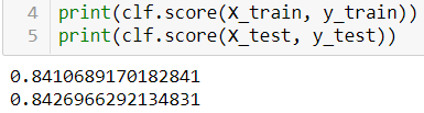
Now after the clf model has been trained well, we can try to print out the accuracy score like this:
And then I found that the model gets the accuracy of 84% on both train and test data. According to this result, we can say that this logistic regression classifier is not overfitting, even though the accuracy itself might still able to be improved using some other techniques.
Model evaluation
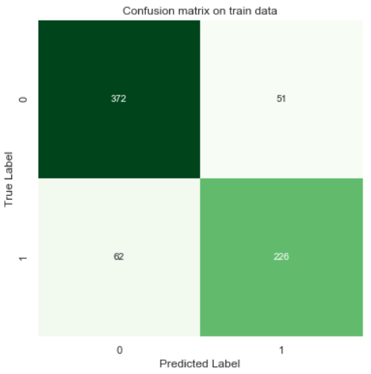
In the model evaluation chapter, we are gonna see more clearly how the predictions distribution looks like. Here I would like to display 2 confusion matrices in which the first one is going to display train data predictions and the next one is used to show the test data predictions.
Let’s start creating the first one. To do that, we need to predict our train data itself and store the predictions in train_preds variable.
train_preds = clf.predict(X_train)
Next, I can simply use confusion_matrix() function to construct a confusion matrix. Remember that the first argument should be the actual values and then followed by the predictions in the next one.
cm = confusion_matrix(y_train, train_preds)
As the cm array has been created, now we can use its value to be displayed using heatmap() function coming from Seaborn module.
What we actually see in the figure above is how the data is predicted. For example, here we got 62 survived passengers which are predicted as not survived. Also , we found here that there are 51 not survived passengers yet predicted as survived.
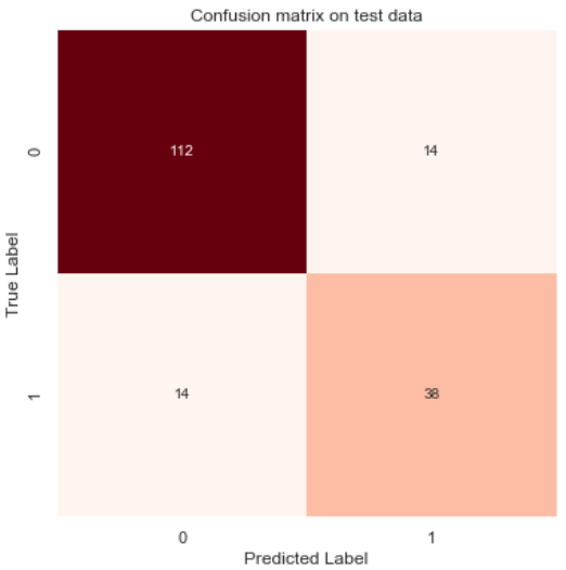
By doing the same thing, we can also display the confusion matrix which is constructed based on predictions on test data (except here I replace plt.cm.Greens with plt.cm.Reds).
Confusion matrix on test data.
And that’s all! I’m pretty sure that 84% of accuracy that I obtain can not be considered as the best one. So I hope you are able to find a technique which can improve the model accuracy. It can probably be achieved by applying more advanced feature engineering or using other machine learning algorithms.
Thanks for reading! Feel free to leave a comment if you find any mistake in this article!
Hi everyone, Ardi here! In this article I wanna do Exploratory Data Analysis (EDA) on Titanic dataset. So far, I’ve been doing several projects in which most of those are related to classification on unstructured data (i.e. image classification). Today, instead of doing the similar project, I wanna try to work with structured data which I think this one is more related to the field of data science in general. Here I decided to use Titanic dataset. The main goal of working with this bunch of data is to perform prediction whether a passenger was survived based on given attributes that they have. The dataset itself can be downloaded here. It should not take long as it only consists of some tiny csv files.
Now after the download finishes we can start to write some code. As usual, I will begin with some imports. By the way I use the combination between Matplotlib and Seaborn just because I’ve been familiar with Matplotlib’s codes while on the other hand I like the figure styles of Seaborn better.
import pandas as pd
import numpy as np
import matplotlib.pyplot as plt
import seaborn as sns; sns.set()
Next, we will load and display the training data. In this EDA I decided not to take into account the data from test set because it does not mention the survival status of the passengers.
df = pd.read_csv(‘train.csv’)
df.head()
The first 5 passengers data.
Data shape, Data types and NaN values
As the data has been loaded, I wanna find out the size of this data frame using df.shape command, which the result indicates that our train.csv contains 891 rows (each representing a passenger) and 12 columns (the attributes of each passenger).
(891, 12)
Big Data Jobs
The datatypes of each column can also be shown by taking the dtypes attribute of df (just by running df.dtypes).
PassengerId      int64
Survived         int64
Pclass           int64
Name            object
Sex             object
Age            float64
SibSp            int64
Parch            int64
Ticket          object
Fare           float64
Cabin           object
Embarked        object
dtype: object
We can see here that there are int64, float64 and object. Well the first two simply means integers and floats respectively, while the object itself is essentially just a string. In the feature engineering chapter we are going to convert all these strings into numbers as basically any machine learning algorithms can only work with numerical data.
Next, I wanna check whether the our data frame df contains NaN (Not a Number) values, which can be done like this:
df.isnull().sum()
The code above displays the following output. Here we can see the number of missing attributes in each column. Well, those missing values may cause a problem — for sure — and we will fix this in the next chapter.
PassengerId      0
Survived         0
Pclass           0
Name             0
Sex              0
Age            177
SibSp            0
Parch            0
Ticket           0
Fare             0
Cabin          687
Embarked         2
dtype: int64
Number of survived vs not survived passengers
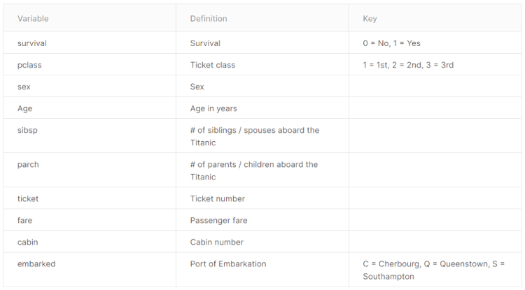
Before I go any further, I wanna show you the details of this Titanic dataset.
According to the table above, it shows that the values of Survived column are either 0 or 1, where 0 represents that the passenger is not survived while 1 says that they are survived. Now in order to find out the number of the two, we are going to employ groupby() method like this:
Here’s how to read it: “Group the data frame by values in Survived column, and count the number of occurrences of each group.”
In this case, since the Survived only has 2 possible values (either 0 or 1), then the code above produces two groups. If we print out survived_count variable, it will produce the following output:
Survived
0    549
1    342
Name: Survived, dtype: int64
Based on the output above, we can see that there are 549 people who were not survived. To make things look better, I wanna display these numbers in form of graph. Here I will use bar() function coming from Matplotlib module. The function is pretty easy to understand. The two parameters that we need to pass is just the index name and its values.
plt.figure(figsize=(4,5))
plt.bar(survived_count.index, survived_count.values)
plt.title('Grouped by survival')
plt.xticks([0,1],['Not survived', 'Survived'])
for i, value in enumerate(survived_count.values):
    plt.text(i, value-70, str(value), fontsize=12, color='white',
             horizontalalignment='center', verticalalignment='center')
plt.show()
And here is the output:
Number of survived and not survived passengers.
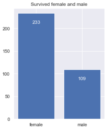
Now I will also do the similar thing in order to find out the number of survived persons based on their gender. Notice that here I use sum() instead of count() because we are only interested to calculate the number of survived passengers which are represented by number 1. So it’s kinda like adding 1s in each group.
plt.figure(figsize=(4,5))
plt.bar(survived_sex.index, survived_sex.values)
plt.title('Survived female and male')
for i, value in enumerate(survived_sex.values):
    plt.text(i, value-20, str(value), fontsize=12, color='white',
             horizontalalignment='center', verticalalignment='center')
plt.show()
Number of survived females and males.
Well, I think the graph above is pretty straightforward to understand 🙂
Ticket class, gender and embarkation distribution
Next, I wanna find out the distribution of ticket classes where the attribute is stored at Pclass column. The way to do it is pretty much similar to the one I created earlier.
Now that there are 3 values stored in pclass_count variable in which each of those represents the number of tickets in each class. However, instead of printing out a graph here I prefer to display it in form of pie chart using pie() function.
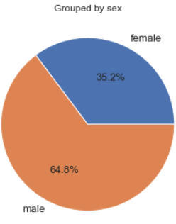
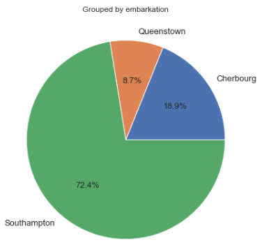
Furthermore, we can also display gender and embarkation distribution pie chart using the exact same method.
Gender distribution shown in percent.Embarkation distribution shown in percent.
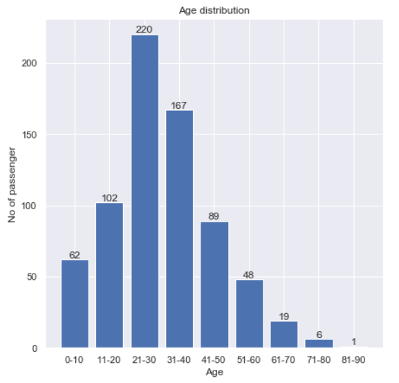
Age distribution
Another thing that I wanna find out is the age distribution. Before I go further, remember that our Age column contains 177 missing values out of 891 data in total. Therefore, we need to get rid of those NaNs first. Here’s my approach to do it:
ages = df[df['Age'].notnull()]['Age'].values
What I am actually doing in the code above is just to retrieve all non-NaN age values and then store the result to ages Numpy array. Next, I will use histogram() function taken from Numpy module. Notice that here I pass two arguments to the function: ages array and a list of bins.
It’s important to know that the output value of np.histogram() function above is a tuple with 2 elements, where the first one holds the number of data in each bin while the second one is the bins itself. To make things clearer in the figure, I will also define labels in ages_hist_labels.
plt.figure(figsize=(7,7))
plt.title('Age distribution')
plt.bar(ages_hist_labels, ages_hist[0])
plt.xlabel('Age')
plt.ylabel('No of passenger')
for i, bin in zip(ages_hist[0], range(9)):
    plt.text(bin, i+3, str(int(i)), fontsize=12,
             horizontalalignment='center', verticalalignment='center')
plt.show()
Age distribution.
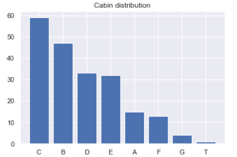
Cabin distribution
If we pay attention to our Cabin column, we can see that all non-NaN values are always started with a capital letter which then followed by several numbers. This can be checked using df[‘Cabin’].unique()[:10] command. Here I only return the first 10 unique values for simplicity.
I got a feeling that probably these initial letters might contain something important, so then I decided to take it and leave the numbers. In order to do that, we need to create a function called take_initial().
def take_initial(x):
    return x[0]
The function above is pretty straightforward though. The argument x essentially represents a string of each row in which we will return only its initial character. Before applying the function to all rows in the Cabin column, we need to drop all NaN values first and store it in cabins object like this:
cabins = df['Cabin'].dropna()
Now as the null values have been removed, we can start to apply the take_initial() function and directly updating the contents of cabins:
cabins = cabins.apply(take_initial)
Next we will use value_counts() method to find out the number of occurrences of each letter. I will also directly store its values in cabins_count object.
cabins_count = cabins.value_counts()
cabins_count
After running the code above we are going to see the following output.
C    59
B    47
D    33
E    32
A    15
F    13
G     4
T     1
Name: Cabin, dtype: int64
Finally, to make things look better, I will use plt.bar() again to display it in form of bar chart.
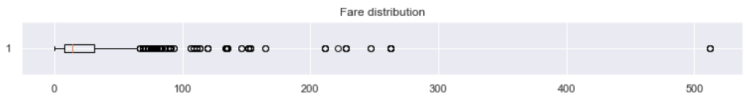
Fare attributes might also play an important role to predict whether a passenger is survived. Different to the previous figures, here instead of using bar or pie chart, I will create a boxplot. Fortunately, it’s extremely simple to do that as basically it can be shown just by using plt.boxplot() function.
Here we see that the distribution is skewed to the right (a.k.a. positive skew) due to the fact that the longer tail is located at the right part of the box, where most of the data points are spread more densely at the range of approximately 10 to 35 currency unit. Additionally, outliers in the samples are represented by the circles. We can also see the fare distribution details using df[‘Fare’].describe() command, which the output is going to look something like this:
count    891.000000
mean      32.204208
std       49.693429
min        0.000000
25%        7.910400
50%       14.454200
75%       31.000000
max      512.329200
Name: Fare, dtype: float64
That’s pretty much about the EDA of Titanic dataset. In the next chapter I am going to do some feature engineering on this data frame. See you there!
Regularization techniques are crucial for preventing your models from overfitting and enables them perform better on your validation and test sets. This guide provides a thorough overview with code of four key approaches you can use for regularization in TensorFlow.


