Musical Instrument Sound Classification using CNN (Part 2/2)

Photo by Jacek Dylag on Unsplash

Hello world, welcome to the second part!

In the previous part, I wrote about data collection and data generation. Here in this part I wanna continue with features preprocessing, label preprocessing, model training and model evaluation respectively. Let’s get started!

Step 3: Features preprocessing (using MFCC)

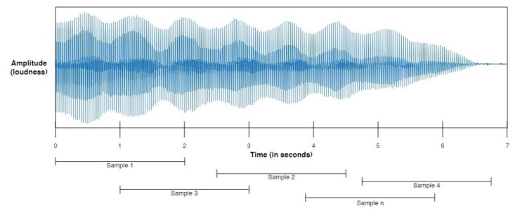
Raw audio wave that we extracted in step 1 using librosa is not really informative since it essentially only consists of one-dimensional data stored in an array. This array shape only represents the amplitude (loudness) of each bit. In fact, loudness is not the only feature that we want to take into account when we are about to distinguish different sounds. Instead, it is also necessary to consider the pitch of those audios. Therefore, in order to extract the pitch information based on given raw audio we are going to utilize a function called mfcc().

MFCC stands for Mel Frequency Cepstral Coefficients. There are so many papers out there related to sound classification and speech recognition which use this feature extraction method in order to obtain more information within audio data. In this article I will be more focusing on how the code work (since the math behind MFCC is very complicated — well, at least for me, lol). If you want to understand more about how to calculate MFCC I recommend you to read it from this page: https://haythamfayek.com/2016/04/21/speech-processing-for-machine-learning.html.

Anyway, remember our generated_audio_waves variable? Since it contains all the raw audio data, then we can simply use a for loop to iterate through all the values of the array and convert each of the waves into MFCC features. Here is my code for that:

mfcc_features = list()
for i in tqdm(range(len(generated_audio_waves))):
mfcc_features.append(mfcc(generated_audio_waves[i]))
mfcc_features = np.array(mfcc_features)

Trending AI Articles:

1. Machine Learning Concepts Every Data Scientist Should Know

2. AI for CFD: byteLAKE’s approach (part3)

3. AI Fail: To Popularize and Scale Chatbots, We Need Better Data

4. Top 5 Jupyter Widgets to boost your productivity!

Now that the MFCC features of all generated data are just stored in mfcc_features variable. If we check the shape before and after processing using mfcc() function like this:

print(generated_audio_waves.shape)
print(mfcc_features.shape)

Then, the output will be (5971, 44100) and (5971, 275, 13) respectively. It is pretty clear that the shape of generated_audio_waves represents the number of samples and the length of each audio samples in bits, in which 44100 is equivalent to 2 seconds. Now the shape of mfcc_features represents the number of audio data and the heatmap image with the size of 275 times 13 produced using mfcc() function. If you try to run the code below you will be able to compare the raw audio data with the MFCC-processed audio:

plt.figure(figsize=(12,2))
plt.plot(generated_audio_waves[30])
plt.title(generated_audio_labels[30])
plt.show()
plt.figure(figsize=(12, 2))
plt.imshow(mfcc_features[30].T, cmap='hot')
plt.title(generated_audio_labels[30])
plt.show()

In the code above I try to display 30th generated audio data, both the raw wave and its MFCC features, in which the outputs are the following two images. Notice the transpose (T) attribute that I apply on the MFCC features data. It is used because by default because mfcc() function outputs time step on its y-axis which makes us harder to compare the raw audio with its extracted features.

Raw audio of saxophone sound.
MFCC features of the saxophone sound displayed in form of heatmap.

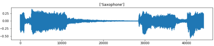
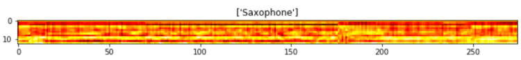
Well, it is quite difficult to interpret the MFCC features. But, the point is that, the heatmap image shows the frequency distribution within each time step where darker pixel represents lower energy and the lighter one shows higher energy. In fact, we can barely see that the silent part of the raw audio data (somewhere between bit number 15000 and 28000) gives slightly darker line on MFCC features approximately at timestep number 75 to 175. In the end of the day, we are going to perform classification on such heatmap images, so, it will be quite similar to image classification tasks in general.

We already got several variables by this far. Now, the two that we are going to use for model training are only mfcc_features (think of this as the X) and generated_audio_labels which contains all the labels (y) of each sample. In the next several steps we are going to actually train the model using these two variables (of course after encoding the label).

Big Data Jobs

Step 4: Target/label preprocessing

Before constructing the neural network architecture, we still need to label-encode and one-hot-encode the labels of each sample. Remember that the values in our generated_audio_labels array are still in form of raw categorical data (i.e. cello, saxophone, acoustic guitar, double bass and clarinet), which is absolutely not acceptable by neural network. Therefore, my approach here is to utilize LabelEncoder() and OneHotEncoder() object coming from Sklearn module. The code implementation can be seen here:

label_encoder = LabelEncoder()
label_encoded = label_encoder.fit_transform(generated_audio_labels)
print(label_encoded)

Now if we try to print out the values of label_encoded, we will get the following output:

array([2, 1, 1, ..., 1, 3, 0])

It seems like that the encoding is working properly. But in fact, this is not acceptable by OneHotEncoder() object. The way to fix this problem is to modify its shape like this:

label_encoded = label_encoded[:, np.newaxis]
label_encoded

Now that label_encoded is ready to be one-hot-encoded as it is already shaped like the following:

array([[2],
[1],
[1],
...,
[1],
[3],
[0]])

Next, the values of label_encoeded will be converted into one hot representation. Things are getting extremely simple when I use OneHotEncoder() object that I don’t even need to iterate through all labels manually. The implementation is quite similar to LabelEncoder().

one_hot_encoder = OneHotEncoder(sparse=False)
one_hot_encoded = one_hot_encoder.fit_transform(label_encoded)
one_hot_encoded

After running the code above, we should get an output like below.

array([[0., 0., 1., 0., 0.],
[0., 1., 0., 0., 0.],
[0., 1., 0., 0., 0.],
...,
[0., 1., 0., 0., 0.],
[0., 0., 0., 1., 0.],
[1., 0., 0., 0., 0.]])

Step 5: Model training (using CNN)

Before training the model, I convert mfcc_features and one_hot_encoded into X and y respectively to make things look more intuitive. Next, I also normalize the values of all samples using standard normalization formula. Lastly, the data are split into train and test in which the test size is taken from 20% of the entire dataset. This train-test split is important to find out whether our model suffers overfitting. Below is the implementation of that:

X = mfcc_features
y = one_hot_encoded
X = (X-X.min())/(X.max()-X.min())
X_train, X_test, y_train, y_test = train_test_split(X, y, test_size=0.2)

Now, the input shape of the neural net is defined as follows:

input_shape = (X_train.shape[1], X_train.shape[2], 1)

If you try to print out that input_shape, the result will be (275, 13, 1). Notice that the number 1 in the shape (last shape axis) should be there because it is just what is expected by Conv2D() layer in our neural network. Hence, we also need to reshape both X_train and X_test to be in that shape as well.

X_train = X_train.reshape(X_train.shape[0], X_train.shape[1], X_train.shape[2], 1)
print(X_train.shape)
X_test = X_test.reshape(X_test.shape[0], X_test.shape[1], X_test.shape[2], 1)
print(X_test.shape)

When you run the code above, you will have the output of (4776, 275, 13, 1) and (1195, 275, 13, 1) respectively. Here we know that we got 4776 samples for training and 1195 samples for testing.

Now it’s time to actually build the Convolutional Neural Network (CNN) classifier. The reason why I use CNN is because this architecture is usually considered as one of the best — if it is not the best — to solve image classification task. And in our case here, the images are in form of heatmap like what I displayed earlier. The complete architecture implementation is shown below along with the loss function and optimizer.

model = Sequential()
model.add(Conv2D(16, (3, 3), activation='relu', strides=(1, 1), 
padding='same', input_shape=input_shape))
model.add(Conv2D(32, (3, 3), activation='relu', strides=(1, 1),
padding='same'))
model.add(MaxPool2D((2, 2)))
model.add(Dropout(0.5))
model.add(Flatten())
model.add(Dense(128, activation='relu'))
model.add(Dropout(0.5))
model.add(Dense(64, activation='relu'))
model.add(Dropout(0.5))
model.add(Dense(5, activation='softmax'))

model.compile(loss='categorical_crossentropy',
optimizer='adam',
metrics=['acc'])

It might be important to keep in mind that categorical cross entropy loss function is used in this case because we are dealing with multiclass classification. Whereas, Adam optimizer is also chosen because I think it is just the best one right now.

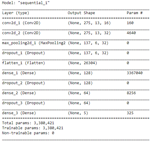
When we run model.summary(), the details of this architecture appears like the following figure. We can see here that the number of params is pretty large.

The CNN architecture that we are going to use for this classification task.

After compiling the model, now our CNN is ready to train. Here I decided to go with 30 epochs, which hopefully will be enough to obtain high accuracy. I ran the code below to start training the model. Also, note that I put the entire training process into history variable which will be useful to track the progress.

history = model.fit(X_train, y_train, epochs=30, validation_data=(X_test, y_test))

And below is how the process goes. I skipped most of those epochs to make things look tidier. By the way it took my computer around 5 minutes to fit the model. Be patient!

Train on 4768 samples, validate on 1192 samples
Epoch 1/30
4768/4768 [==============================] - 10s 2ms/step - loss: 1.4365 - acc: 0.3473 - val_loss: 1.1578 - val_acc: 0.5529
.
.
.
Epoch 10/30
4768/4768 [==============================] - 7s 1ms/step - loss: 0.6428 - acc: 0.7664 - val_loss: 0.5620 - val_acc: 0.8020
.
.
.
Epoch 20/30
4768/4768 [==============================] - 7s 1ms/step - loss: 0.4469 - acc: 0.8349 - val_loss: 0.4510 - val_acc: 0.8582
.
.
.
Epoch 30/30
4768/4768 [==============================] - 7s 1ms/step - loss: 0.3470 - acc: 0.8729 - val_loss: 0.3962 - val_acc: 0.8842

Well, after several minutes of waiting, finally we got the final result. We can see here that the accuracy scores in the last epoch are 87% and 88% towards training and testing data respectively.

We can also see the improvement of the model goes at every epoch using Matplotlib to make things look clearer. The code below is used to display both loss value decrease and accuracy score improvement.

plt.figure(figsize=(8,8))
plt.title(‘Loss Value’)
plt.plot(history.history[‘loss’])
plt.plot(history.history[‘val_loss’])
plt.legend([‘loss’, ‘val_loss’])
print(‘loss:’, history.history[‘loss’][-1])
print(‘val_loss:’, history.history[‘val_loss’][-1])
plt.show()
plt.figure(figsize=(8,8))
plt.title('Accuracy')
plt.plot(history.history['acc'])
plt.plot(history.history['val_acc'])
plt.legend(['acc', 'val_acc'])
print('acc:', history.history['acc'][-1])
print('val_acc:', history.history['val_acc'][-1])
plt.show()

And the output looks something like the two images below.

Loss value decrease of both train and test data.
Accuracy score improvement of both train and test data.

According to the two graphs above, we can see that our model is performing pretty well as it reaches the final accuracy of 87% and 88% towards train and test data respectively. Also, both loss values are also decreasing as the the number of epoch increases. Therefore, we can conclude that this CNN classifier does not suffer overfitting at all!

Step 6: Model evaluation

Now let’s get deeper into the CNN model. In order to evaluate the performance of the model better, we are going to predict both train and test data again, but in a different session with the training process. Here I would like to start predicting the test data first.

predictions = model.predict(X_test)

After running the code above, now predictions variable holds all the predicted class of each sample in X_test, but still in form of probability values. For example prediction values of the first sample (predictions[0]) looks like this:

array([3.0511815e-06, 2.2099694e-05, 9.9997330e-01, 1.0746862e-12,
1.5381156e-06], dtype=float32)

What it actually says is that the class of index 2 holds the highest probability since it has the score of >0.9 while other indices only has <0.1 score. Hence, the prediction of this sample falls to class [0, 0, 1, 0, 0]. Now if we take the argmax of that array, we are going to obtain the value of 2, where this number represents the sound of a clarinet.

The code below shows how to take the argmax of all predictions on X_test and then followed by decoding y_test into the same form as the predictions variable (because previously we already converted y_test into one-hot representation, now we need to convert that back to label-encoded form). This is extremely necessary to do because we want to compare each of the element of predictions and y_test.

predictions = np.argmax(predictions, axis=1)
y_test = one_hot_encoder.inverse_transform(y_test)

As predictions and y_test are now comparable, we can start to create a confusion matrix to evaluate the model performance better. Here we are going to use confusion_matrix function taken from Sklearn module. The implementation looks like this:

cm = confusion_matrix(y_test, predictions)
plt.figure(figsize=(8,8))
sns.heatmap(cm, annot=True, xticklabels=label_encoder.classes_, yticklabels=label_encoder.classes_, fmt='d', cmap=plt.cm.Blues, cbar=False)
plt.xlabel('Predicted Label')
plt.ylabel('True Label')
plt.show()

After running the code above, we should get an output like the following image:

Confusion matrix on test data.

Using the confusion matrix above, we are able to know which class makes our CNN confused. Let’s take a look at saxophone true label (last row). Here we can see that 186 samples are predicted correctly, while 20 other saxophone samples are predicted as clarinet. Hence, we can guess that probably our classifier sometimes get difficulty to distinguish the sound of saxophone and clarinet.

That’s all of musical instrument sound classification project. I hope you learn something new from this article. See you in the next one!

And here is the code I promised earlier:)

Don’t forget to give us your ? !


Musical Instrument Sound Classification using CNN (Part 2/2) was originally published in Becoming Human: Artificial Intelligence Magazine on Medium, where people are continuing the conversation by highlighting and responding to this story.

Via https://becominghuman.ai/musical-instrument-sound-classification-using-cnn-part-2-2-aaa668a3862a?source=rss—-5e5bef33608a—4

source https://365datascience.weebly.com/the-best-data-science-blog-2020/musical-instrument-sound-classification-using-cnn-part-22

Natural Language Processing for WhatsApp Chats

Natural Language Processing or NLP is a field of Artificial Intelligence which focuses on enabling the systems for understanding and…

Via https://becominghuman.ai/natural-language-processing-for-whatsapp-chats-67f0b902afbc?source=rss—-5e5bef33608a—4

source https://365datascience.weebly.com/the-best-data-science-blog-2020/natural-language-processing-for-whatsapp-chats

Computer Vision TutorialLesson 3

source https://365datascience.weebly.com/the-best-data-science-blog-2020/computer-vision-tutoriallesson-3

Top Google AI Machine Learning Tools for Everyone

Google is much more than a search company. Learn about all the tools they are developing to help turn your ideas into reality through Google AI.

Originally from KDnuggets https://ift.tt/314ChFA

source https://365datascience.weebly.com/the-best-data-science-blog-2020/top-google-ai-machine-learning-tools-for-everyone

How Anonymous is Anonymized Data?

As the collection of personal data democratized over the previous century, the question of data anonymization started to rise. The regulations coming into effect around the world sealed the importance of the matter.

Originally from KDnuggets https://ift.tt/3172e7F

source https://365datascience.weebly.com/the-best-data-science-blog-2020/how-anonymous-is-anonymized-data

Top Stories Aug 10-16: Know What Employers are Expecting for a Data Scientist Role in 2020; The List of Top 10 Lists in Data Science

Also: 5 Different Ways to Load Data in Python; Facebook Uses Bayesian Optimization to Conduct Better Experiments in Machine Learning Models; Exploring GPT-3: A New Breakthrough in Language Generation; Unit Test Your Data Pipeline, You Will Thank Yourself Later; Going Beyond Superficial: Data Science MOOCs with Substance

Originally from KDnuggets https://ift.tt/324M5i6

source https://365datascience.weebly.com/the-best-data-science-blog-2020/top-stories-aug-10-16-know-what-employers-are-expecting-for-a-data-scientist-role-in-2020-the-list-of-top-10-lists-in-data-science

Reducing Re-Identification Risk in Health Data

Want to learn more about our recommendations for strengthening privacy while preserving utility? Read Immuta’s new whitepaper, “Reducing Re-Identification Risk in Health Data: A Guide to Three Privacy Enhancing Technologies”, to get the inside scoop on the best privacy enhancing technologies.

Originally from KDnuggets https://ift.tt/3h7bNZB

source https://365datascience.weebly.com/the-best-data-science-blog-2020/reducing-re-identification-risk-in-health-data

Musical Instrument Sound Classification using CNN (Part 1/2)

Photo by Michal Czyz on Unsplash

Hello world! It’s been pretty long since my last post. Previously, I was talking about digit reconstruction using deep autoencoder, which the article can be seen down here.

The Deep Autoencoder in Action: Digit Reconstruction

Anyway, in this article I would like to share another project that I just done: classifying musical instrument based on its sound using Convolutional Neural Network (CNN). Below is the list of what we need to do:

  1. Data collection
  2. Data generation
  3. Features preprocessing (using MFCC)
  4. Label preprocessing
  5. Model training (using CNN)
  6. Model evaluation

Well, I think there is no much thing to say anymore for the intro, so now let’s just jump into the project!

Note: I attach the full code in the end of the last chapter!

Jobs in AI

Step 1: Data collection

As always, the first thing I do when working with machine learning or deep learning projects is collecting all required data. Today, I am taking thousands of audio files from a Kaggle competition which you can download from this link: https://www.kaggle.com/c/freesound-audio-tagging/data. The dataset contains 41 classes in which each of those represents the name of a musical instrument such as cello, chime and clarinet. Actually there are also some other non-musical instrument sounds like telephone and fireworks in the dataset. However, here in my project I decided to choose only 5 musical instruments to be classified for simplicity.

Now let’s start with importing all required modules:

import os
import librosa
import pickle
import numpy as np
import pandas as pd
import matplotlib.pyplot as plt
import seaborn as sns
from tqdm import tqdm
from python_speech_features import mfcc
from sklearn.preprocessing import LabelEncoder, OneHotEncoder
from sklearn.model_selection import train_test_split
from sklearn.metrics import confusion_matrix
from keras.layers import Conv2D, MaxPool2D, Flatten, Dense, Dropout
from keras.models import Sequential

Here I would like to highlight several imports that you probably might still not familiar with, those are: librosa, tqdm and mfcc. First, librosa is a Python module which I use to load all audio data. Next, tqdm is actually not very necessary, I just like to use it to display progress bar in a loop operation. Lastly, mfcc is a function coming with python_speech_features module which is very important to extract audio features to make those audio wave data more informative.

The next step is to load train.csv in form of a pandas data frame using the following code.

df = pd.read_csv('train.csv')
df.head()

Below is how the data frame looks like. You can see here that it contains filename-label pair and manually_verified column which I guess it’s used to tag whether an audio clip is verified by a real person.

Content of train.csv file.

As I’ve mentioned earlier, in this project I will only use 5 out of 41 classes in the dataset. Those classes are Cello, Saxophone, Acoustic_guitar, Double_bass and Clarinet. Here is how to filter out those classes.

df = df[df['label'].isin(['Cello','Saxophone','Acoustic_guitar','Double_bass', 'Clarinet'])]

Trending AI Articles:

1. Machine Learning Concepts Every Data Scientist Should Know

2. AI for CFD: byteLAKE’s approach (part3)

3. AI Fail: To Popularize and Scale Chatbots, We Need Better Data

4. Top 5 Jupyter Widgets to boost your productivity!

If you check the shape of the data you will find that the number of data is now only 1500 (previously there are 9473 files). As the data already filtered to only 5 classes, we will load those actual audio files using the following approach:

path = 'audio_train/'
audio_data = list()
for i in tqdm(range(df.shape[0])):
audio_data.append(librosa.load(path+df['fname'].iloc[i]))
audio_data = np.array(audio_data)

Well, this process is relatively simple yet it takes several minutes to run. Here I declared an empty list called audio_data and append each of raw audio data using librosa.load() function. Keep in mind that the shape of this audio_data variable is (1500, 2) in which the first axis represents the number of raw audio waves and the second axis represents 2 columns (which stores audio waves and sample rate respectively). Lastly, I also convert the audio_data list into Numpy array.

By the way, if you use tqdm() function like what I did, you will have the output which looks something like this:

tqdm() function in action.

Now we will put the content of audio_data variable into data frame df which can be done using the following code:

df['audio_waves'] = audio_data[:,0]
df['samplerate'] = audio_data[:,1]
df.head()

Then it will show an output which looks like this:

Our data frame with new column: audio_waves and samplerate.

Notice that the index number of the data frame is unordered. This is because we only take rows which contains the 5 labels I chose earlier. And fortunately for this case it’s completely fine to be like that.

Now, what I wanna do is to create 2 new columns which will store the length of each audio file, both in bits and seconds. Here is my approach:

bit_lengths = list()
for i in range(df.shape[0]):
bit_lengths.append(len(df['audio_waves'].iloc[i]))
bit_lengths = np.array(bit_lengths)
df['bit_lengths'] = bit_lengths
df['seconds_length'] = df['bit_lengths']/df['samplerate']
df.head()

I think the code above is pretty straightforward, I am sure you can understand it easily without further explanation.

Anyway, the two new columns are called bit_lengths and second_lengths. bit_lengths is essentially just the number of bits in each audio waves, while second_lengths is the length of all audio files in seconds. We can think of samplerate column like the number of frames in a video. Hence, in order to get the value for second_lengths, we can simply divide the number of all bits of each audio wave with the corresponding sample rate.

Now our data frame also contains the length of each audio file.

Step 2: Data generation

Up to this point, we already got a data frame df which now contains the length of all audio files. We just realized that actually all those audios are having different lengths. And well, this is a problem. Why? Because any machine learning or deep learning classifier models only accept data with exact same shape for each sample. So now, the solution is to make those data having the same length. In this project, I decided to go with 2 seconds of audio data.

In order to do it, the first thing I wanna do is to drop all samples which are shorter than 2 seconds. Here is the code to do it:

df = df[df['second_lengths'] >= 2.0]

Pretty simple isn’t it? Now if you check the number of data using df.shape, then you will have the shape of (1306, 7). You can see here that approximately 200 of our audio files are dropped thanks to this operation since those audios must be shorter than 2 seconds in length.

I use the code below to check whether we already eliminated audio files that have less than 2 seconds length.

min_bits = np.min(df['bit_lengths'])
print(min_bits)
min_seconds = np.min(df['second_lengths'])
print(min_seconds)

Both prints gives 44100 and 2.0 which represents the shortest audio file in the data frame in bits and seconds respectively.

We already done plenty of things as of this stage. Here I decided to make a checkpoint so that I don’t have to go through all those loadings if I want to run this code again in the future. So what I wanna do now is to utilize pickle module, which is very useful to store any kind of variables into separate file. And here in my case I want to store the data frame df into a file called audio_file.pickle. Below is the code for that.

with open('audio_df.pickle', 'wb') as f:
pickle.dump(df, f)

Now assume that you’re now in the future and you want to reload the variable, you can do it simply by using the following code:

with open('audio_df.pickle', 'rb') as f:
df = pickle.load(f)

That’s it! Now you got the exact same data frame (also stored in variable df) as what you saved in the past.

Anyway, that was just a way to create a checkpoint. If you feel like you don’t need one, just skip that part.

Okay, so actually I haven’t finished explaining about the entire part of data generation. Now what I wanna do next is to do what’s so-called as random sampling method — well, at least that’s how I call it.

Data generation using random sampling method on audio waves.

So this random sampling works by taking n samples, where n is a number that we are free to choose. In this case, I want all those samples to have 2-seconds length. This 2-seconds audio chunk is taken at any position within an audio file in which the audio file itself is also selected randomly within the dataset for each iteration. Below is my implementation for this.

num_samples = 6000
generated_audio_waves = list()
generated_audio_labels = list()
for i in tqdm(range(num_samples)):
try:
chosen_file = np.random.choice(df['fname'].values)
chosen_initial = np.random.choice(np.arange(0,df[df['fname']==chosen_file]['bit_lengths'].values-min_bits))
generated_audio_waves.append(df[df['fname']==chosen_file]['audio_waves'].values[0][chosen_initial:chosen_initial+min_bits])

generated_audio_labels.append(df[df['fname']==chosen_file]['label'].values)
except ValueError:
continue
generated_audio_waves = np.array(generated_audio_waves)
generated_audio_labels = np.array(generated_audio_labels)

Well, the point of the code above is to generate 2-seconds length audio in which it is stored in generated_audio_waves (for the wave data itself) and generated_audio_labels (for the labels of the corresponding wave data). Here I decided to take 6000 audio chunks which I declared using num_samples variable. Next, after generating all data, I also convert both lists to Numpy array because I think it’s just simpler than Python list.

Probably you might be wondering why I put try-except command in the code. And well, to be honest I completely got no idea why at certain iteration it always returns error. So, in order to handle that error, I just put a try-except command there and fortunately it only skips little number of data, which I think it doesn’t really affect the neural network model performance in the end.

Alright, I think I have to stop right now since I feel like this article has been very long. And, yea, this is the end of the first part of this project. I will continue explaining the next processes in part 2 (features preprocessing, label preprocessing, model training and model evaluation). See you there!

Don’t forget to give us your ? !


Musical Instrument Sound Classification using CNN (Part 1/2) was originally published in Becoming Human: Artificial Intelligence Magazine on Medium, where people are continuing the conversation by highlighting and responding to this story.

Via https://becominghuman.ai/musical-instrument-sound-classification-using-cnn-part-1-2-43197e554cc8?source=rss—-5e5bef33608a—4

source https://365datascience.weebly.com/the-best-data-science-blog-2020/musical-instrument-sound-classification-using-cnn-part-12

3D Human Pose Estimation Experiments and Analysis

In this article, we explore how 3D human pose estimation works based on our research and experiments, which were part of the analysis of applying human pose estimation in AI fitness coach applications.

Originally from KDnuggets https://ift.tt/3g1W24V

source https://365datascience.weebly.com/the-best-data-science-blog-2020/3d-human-pose-estimation-experiments-and-analysis

Applying Darwinian Evolution to feature selection with Kydavra GeneticAlgorithmSelector

The development of machine learning implies a lot of maths. But sometimes during feature selection phase maths sometimes can’t give an exact answer (because of the structure of data, it’s source, and many other causes). Then in-game enter the Programming tricks, mostly brute force methods :).

Genetic algorithms are a family of algorithms inspired by biological evolution, that basically use the cycle — cross, mutate, try, developing the best combination of states depending on the scoring metric. So, let’s get to the code.

Trending AI Articles:

1. Machine Learning Concepts Every Data Scientist Should Know

2. AI for CFD: byteLAKE’s approach (part3)

3. AI Fail: To Popularize and Scale Chatbots, We Need Better Data

4. Top 5 Jupyter Widgets to boost your productivity!

Using GeneticAlgorithmSelector from Kydavra library.

To install kydavra just write the following command in terminal:

pip install kydavra

Now you can import the Selector and apply it on your data set a follows:

from kydavra import GeneticAlgorithmSelector
selector = GeneticAlgorithmSelector()
new_columns = selector.select(model, df, ‘target’)

As with every Kydavra selector that’s all. Now let’s try it on the Hearth disease dataset.

Jobs in AI
import pandas as pd
df = pd.read_csv(‘cleaned.csv’)

I highly recommend you to shuffle your dataset before applying the selector, because it uses metrics (and right now cross_val_score isn’t implemented in this selector).

df = df.sample(frac=1).reset_index(drop=True)

Now we can apply our selector. To mention it has some parameters:

  • nb_children (int, default = 4) the number of best children that the algorithm will choose for the next generation.
  • nb_generation (int, default = 200) the number of generations that will be created, technically speaking the number of iterations.
  • scoring_metric (sklearn scoring metric, default = accuracy_score) The metric score used to select the best feature combination.
  • max (boolean, default=True) if is set to True the algorithm will select the combinations with the highest score if False the lowest scores will be chosen.

But for now, we will use the basic setting except of the scoring_metric, because we have there a problem of disease diagnosis, so it will better to use Precision instead of accuracy.

from kydavra import GeneticAlgorithmSelector
from sklearn.metrics import precision_score
from sklearn.ensemble import RandomForestClassifier
selector = GeneticAlgorithmSelector(scoring_metric=precision_score)
model = RandomForestClassifier()

So now let’s find the best features. GAS (short version for GeneticAlgorithmSelector) need a sklearn model to train during the process of choosing features, the data frame itself and of course the name of target column:

selected_cols = selector.select(model, df, 'target')

Now let’s evaluate the result. Before feature selection, the precision score of the Random Forest was — 0.805. GAS choose the following features:

['age', 'sex', 'cp', 'fbs', 'restecg', 'exang', 'slope', 'thal']

Which gave the following precision score — 0.823. Which is a good result, knowing that in majority of cases it is very hard to level up the scoring metrics.

If you want to find out more about Genetic Algorithms at the bottom of the article are some useful links. If you tried Kydavra and have some issues or feedback, please contact me on medium or please fill this form.

Made with ❤ by Sigmoid

Useful links:

Don’t forget to give us your ? !


Applying Darwinian Evolution to feature selection with Kydavra GeneticAlgorithmSelector was originally published in Becoming Human: Artificial Intelligence Magazine on Medium, where people are continuing the conversation by highlighting and responding to this story.

Via https://becominghuman.ai/applying-darwinian-evolution-to-feature-selection-with-kydavra-geneticalgorithmselector-f94c885a9ea7?source=rss—-5e5bef33608a—4

source https://365datascience.weebly.com/the-best-data-science-blog-2020/applying-darwinian-evolution-to-feature-selection-with-kydavra-geneticalgorithmselector

Design a site like this with WordPress.com
Get started