365 Data Science is an online educational career website that offers the incredible opportunity to find your way into the data science world no matter your previous knowledge and experience.
Bring your Pandas dataframes to life with D-Tale. D-Tale is an open-source solution for which you can visualize, analyze and learn how to code Pandas data structures. In this tutorial you’ll learn how to open the grid, build columns, create charts and view code exports.
Data is the bread and butter of a Data Scientist, so knowing many approaches to loading data for analysis is crucial. Here, five Python techniques to bring in your data are reviewed with code examples for you to follow.
Artificial Intelligence (AI) technology has already reshaped a lot of industries from hospitality to healthcare and learning. The leading solution is also dramatically transforming the logistics field. According to the research, the global AI in the logistics and supply chain market is expected to grow at a CAGR of 45.5% by 2027. In this article, we’re going to overlook the AI trends in logistics to look for in 2020.
How Artificial Intelligence is transforming the logistics industry
Today more and more AI-based logistics applications appear on the market to optimize the transportation companies’ and business performance. Each solution can help organizations to do certain tasks. So, let’s see 8 ways AI is transforming the logistics industry and how technology can improve your business.
Automated warehouses
Integration of the AI solutions can decrease the costs by automating warehouses. The technology can do a lot of everyday routine tasks and change many processes like data collection, inventory, and so on. AI has the ability to analyze the data gathered, predict demand, re-route in-transit goods, modify orders, and communicate with each other for optimizing transportation between warehouses. Such agility and planning in logistics mean lower costs, better service, faster work.
Jobs in ML
AI-powered big data
It’s not news that big data has great potential in various fields, including transportation and supply chain. There is tons of information gathered daily when dealing with logistics. It’s a true challenge to process and exploit all the data fast and accurately for planning. AI can do that. Besides that, the system considers such factors as political landscape, weather, and others. Today thanks to the AI solutions integrated, logistics companies can:
Refine the data gathered from each touchpoint;
Analyze all the data accurately;
Come up with the patterns for better strategic decision making;
Increase automation of repetitive tasks;
Make clear and accurate predictions.
Autonomous vehicles
Watching movies such as Total Recall with Arnold Schwarzenegger and Demolition Man with Sylvester Stallone, the autonomous vehicles seemed to be just a fantasy. However, it’s a reality nowadays. Currently, such companies as Tesla and Google have already developed self-driving cars with AI implemented.
Autonomous vehicles promise to reduce the costs, save time, decrease accident rates. Currently, human supervision is a must to drive autonomous vehicles on roads, yet in the future it’s expected that cars will be fully automated.
AI-based computer vision can help logistics companies with a wide range of tasks and optimize performance. For instance, the AI computer vision used for automating warehouses can identify the needs and help with organization of the inventory. Another use-case is from logistics giant DHL — visual inspection powered by AI. The technology helps:
Scan and identify the damage;
Classify it by the type;
Determine the appropriate remedial measures.
The key feature of the computer vision in this case is speed. The AI solution does all listed tasks much faster than ever before.
There is one more great example from the retail giant Amazon. The system helps unload a trailer of inventory in only 30 minutes when doing the same without the computer vision takes several hours.
Smart roads
AI used for roads can improve transportation and make it more effective, in-time, and safe. Thus, the great example of the technology used for the purpose are highways with solar panels and LED lights. Thus, the panels provide electricity and LED lights alert about various road conditions. What’s more, solar panels prevent the appearance of the slippery surface on the road in winter.
Drivers, using the roads with AI-based fiber optic sensors, can get the information about the traffic volumes, alerts about road conditions, accidents, etc. In the event that the vehicle or truck gets in an accident on such a road, the AI technology will immediately report appropriate emergency services.
Artificial Intelligence of the back office operations
The AI solutions integrated can automate the repetitive back-office tasks and operations. Combining AI with Robotic Process Automation (RPA), the logistics organizations can improve the accuracy, speed, productivity of the employees, and reduce the costs. The technology is helpful with the everyday data-related tasks that can be done by robotic assistance. This will free your workers and let them focus on other crucial aspects. That leads to a rise in their quality of work.
Predictive capabilities
Accurate predictions can save money and customers. The AI technology integrated provides various algorithms for forecasting the trends, goods, and/or supplies needed for your company in the future. As Deloitte reports, such algorithms forecast outcomes precisely and better than human experts. The technology tracks and measures all inputs and variables for creating contingency plans. That can reduce the costs of your company, navigating you successfully through any emergencies.
Customer experience
It’s no matter if your company is B2B or B2C, it’s crucial to keep your customers engaged. The fastest way to do it is to improve their experience. AI technology can increase customer loyalty and retention. The solution can personalize the service, suggest products according to the previous purchases, page views, and customizations based on the buying preferences, habits. In such a way the AI integration can turn users into consumers, increase revenue, build a brand.
Final thoughts
AI technology dramatically reshapes the logistics field. The integration of the solution can improve inventory, transportation, accuracy, management, and power the employees to make their job more efficient. The key feature of the solution is the automation of the routine tasks, speed, and efficiency of the back office, big data analytics, and on and on. Artificial Intelligence can also eliminate the risks and reduce the accidents associated with the transportation of the cargos. In this article, we provide you with 8 ways the AI transforms the industry and show you the use-cases on how your business can benefit from the integration of the solution.
Hello world! Hope you’re doing great today. In this article I would like to do a project related to Natural Language Processing (NLP). The project itself is not going to be very complicated as what we are gonna do is just a simple binary classification task.
So we know that Coronavirus is still around up until the time when I write this article. And thus, it’s obviously possible that there are also plenty of fake news related to that topic coming into the society. So the objective of this project is to create a machine learning model which is able to detect whether a news is fake or real.
Note: full code available in the end of this article.
Let’s start with some imports. I will explain them later on.
import re
import pandas as pd
import numpy as np
import matplotlib.pyplot as plt
import seaborn as sns
from sklearn.feature_extraction.text import CountVectorizer
from sklearn.naive_bayes import MultinomialNB
from sklearn.model_selection import train_test_split
from sklearn.metrics import confusion_matrix
from nltk.tokenize import word_tokenize
from nltk.corpus import stopwords
Data collection & analysis
Before I go any further, I wanna inform you that the project that I’m going to explain here is inspired by the this article. The author of that article uses logistic regression to do the classification and obtain 93% of accuracy towards test data. On the other hand, here in my project I would like to employ Naïve Bayes classifier instead and see if I can obtain higher accuracy using this approach with the exact same dataset. You can download the COVID-19 news dataset from here.
Now after downloading the dataset, let’s do a simple Exploratory Data Analysis (EDA) to find out important (and probably interesting) things in the dataset.
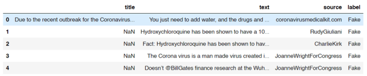
After running the code above, we should get an output like the following image and the shape of the data frame df, which is (1164, 4). It says that our dataset consists of 1164 rows in which each of those has 4 attributes.
How the dataset looks like.
Look at the title column. Here we see that some of the titles are missing. Now I got a feeling that probably there are also some other missing stuff in the dataset which might affect the overall performance of our model. So I decided to count the number of those missing values from each column.
print("No of missing title\t:", df[df['title'].isna()].shape[0])
print("No of missing text\t:", df[df['text'].isna()].shape[0])
print("No of missing source\t:", df[df['source'].isna()].shape[0])
print("No of missing label\t:", df[df['label'].isna()].shape[0])
And here is the result:
No of missing title     : 82
No of missing text      : 10
No of missing source    : 20
No of missing label     : 5
Now we know that actually some of the cells in our data frame contains NaN (Not a Number) values. By knowing this fact, what I wanna do now is assigning an empty string (‘’) to all those cells like this:
df = df.fillna(‘’)
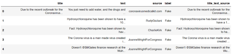
Next, the title, text and source columns are then going to be concatenated which the result is stored in another new column called title_text_source . This new column in our data frame df is going to be our raw X data.
Now our data frame is going to look something like this:
Our data frame now has title_text_source column.
On the other hand, all samples with missing values in label column will just be dropped since I got no idea whether each of those is real or fake news. The following code is my approach to delete them.
Now the output after running the code above shows that all our non-labeled data are already removed as there is no empty string appears as the unique value in label column.
array(['Fake', 'TRUE', 'fake'], dtype=object)
But wait! We got another problem here! You can see the output above that our labels are not uniform. So then it’s really necessary to fix this. Here I decided to put those into 2 classes, namely TRUE and FAKE. Below is the code to do so:
Now that all fake and Fake labels are already converted into FAKE. You can check it by running df[‘label’].unique() again. Since up to this step we already got 2 unique labels (only FAKE and TRUE), we can calculate the number of data of each class using the following code:
After running the code above we should get an output like this:
No of fake data:  575
No of true data:  584
Now we can see here that the numbers of fake and true data are almost equal. And this is a good news because any machine learning algorithm will work best if the number of data of all classes are balanced.
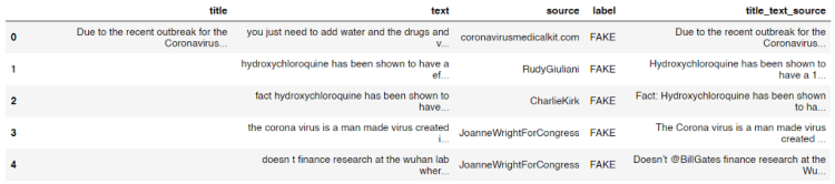
Lemme print out our latest data frame df again using df.head() command.
How our data frame looks like after adding title_text_source column and updating each label.
We know that there are probably plenty of useless words or characters which exist in the title_text_source column, such as Twitter user name and stop words (i.e. and, or, if, the, into, etc). Here in this step we are going to get rid of those words using the clean() function I defined below.
stop_words = set(stopwords.words('english'))
def clean(text):
    # Lowering letters
    text = text.lower()

    # Removing html tags
    text = re.sub(r'<[^>]*>', '', text)

    # Removing twitter usernames
    text = re.sub(r'@[A-Za-z0-9]+','',text)

    # Removing urls
    text = re.sub('https?://[A-Za-z0-9]','',text)

    # Removing numbers
    text = re.sub('[^a-zA-Z]',' ',text)

    word_tokens = word_tokenize(text)

    filtered_sentence = []
    for word_token in word_tokens:
        if word_token not in stop_words:
            filtered_sentence.append(word_token)

    # Joining words
    text = (' '.join(filtered_sentence))
    return text
So the first thing I do in the code above is to create a set of all stop words in English stored in stop_words variable. Next, I define a clean() function which takes a text as the only parameter. After that, this text is going to be processed, mostly using re (Regular Expression) module. You can see the comments in the code for the details. I also perform tokenization to the text in order to filter out stop words before returning the cleaned text as the output.
Before actually applying the function to each rows in the title_text_source column, I want to check whether the function works as expected like this:
print(clean('Hello World 22 Ardi, and or if they 3878, I am @Ardi'))
And yes, it the function works properly as it does remove all unnecessary words.
'hello world ardi'
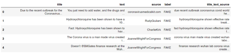
Now, to clean all texts stored in title_text_source column, we can simply use apply() method to that column like this:
After running the code above you will see that all texts in the column are already cleaned.
Now the texts inside title_text_source column are already cleaned.
Count vectorizer
We know that any machine learning or deep learning algorithms can not directly work with words. Thus, it’s obviously necessary to convert all texts in title_text_source into numbers. In this project, I am going to use count vectorizer as the approach to do it. The concept of count vectorizer itself is pretty trivial, since we only need to count the occurrence of each word for every single text in order to create a feature vector of that. If you still don’t get the idea of count vectorizer I recommend you to read this simple explanation.
The implementation is very simple thanks to the existence of Scikit-learn module.
vectorizer = CountVectorizer()
X = vectorizer.fit_transform(df['title_text_source'].values)
X = X.toarray()
Look at the code above. The first thing we do is to initialize a count vectorizer object which I call it as vectorizer. Then in the next two lines I use this vectorizer to convert all values of title_text_source column (which is still in form of text) into array of word occurrences. Now if we try to print out this X variable, we will get the following output:
The shape of the array above is (1159, 21117) which represents the number of samples and the feature vector size of each sample respectively.
Naïve Bayes classifier
Up to this point we already got feature vectors for all samples stored in X variable. To make things more intuitive, I will also define y variable, which I will use it to store all ground truths (a.k.a. labels).
y = df['label'].values
Now we can use y as the replacement of df[‘label’].values
Before training a classifier, we are going to split the data into train and test, where 20% of the entire samples in the dataset are going to be used to test the overall performance of the model. This splitting can easily be done using train_test_split function taken from Sklearn module:
X_train, X_test, y_train, y_test = train_test_split(X, y, shuffle=True, test_size=0.2, random_state=11)
After running the code above, we got 4 new variables which I guess all of those are self-explanatory.
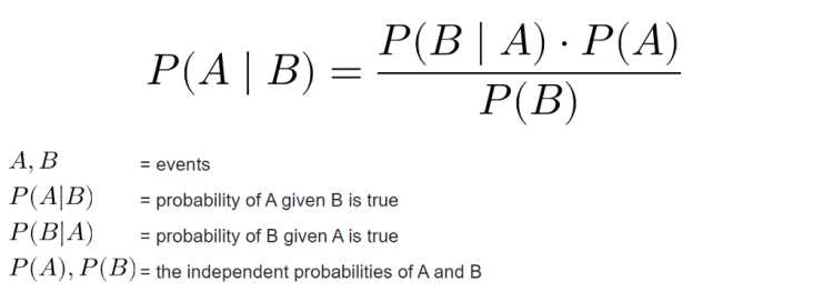
Now as the data already split it’s time to define a model which in this project I will be using Naïve Bayes. Mathematically speaking, this algorithm works by calculating the class (label) prediction probability based on given features (text) of each sample using Bayes’ theorem. If you wanna understand better about the mathematical concept of this algorithm you can open up this page. In my opinion that’s the best site that explains Naïve Bayes in depth.
Bayes’ theorem.
In addition, there are several types of Naïve Bayes algorithm, those are Gaussian, Multinomial and Bernoulli. In this project I will be using Multinomial Naïve Bayes since it’s the best one to be implemented in this text classification task due to its ability to maintain the number of word occurrences in each document. Fortunately, Sklearn provides an easy-to-implement object called MultinomialNB(), so that we don’t have to code the algorithm from scratch.
The code below shows how I train a Multinomial Naïve Bayes classifier on train data:
clf = MultinomialNB()
clf.fit(X_train, y_train)
Next, we can try to calculate the accuracy score of the classifier using score() method.
The output of the code above shows that our model is pretty good! We can see here that the model is slightly overfitting, but I guess it’s still a good one.
Accuracy on train data    : 0.9633225458468176
Accuracy on test data   : 0.9353448275862069
Model evaluation
After training a model, I usually also create a confusion matrix in order to find out the number of misclassified samples in more detail. In order to do so, I need to predict the class of test data first:
predictions = clf.predict(X_test)
Next, we can just compare the values of predictions variable with its ground truth y_test using confusion_matrix() function coming from Sklearn module.
cm = confusion_matrix(y_test, predictions)
Since the return value of confusion_matrix() is essentially a square array, then we can just plot that array using heatmap() function which can be taken from Seaborn module.
We will see the following output after running the code above.
Confusion matrix of our Naïve Bayes model on COVID-19 news dataset.
Now what if we got a new news and we wanna find out whether its news is a fake one? In this part I would like to demonstrate how to perform prediction on new news data. Here I store the text in sentence variable.
sentence = 'The Corona virus is a man made virus created in a Wuhan laboratory. Doesn’t @BillGates finance research at the Wuhan lab?'
We can see the code above that in order to predict new data, we first have to clean the sentence using clean() function I defined in the earlier part of this article. Next, the cleaned sentence is transformed to array of numbers using our vectorizer object, in which in this case it is a CountVectorizer(). Lastly, as the sentence has been converted into vectors, then we are able to predict its class, and in this case the final output is like this:
array(['FAKE'], dtype='<U4')
According to the output above, it shows that the sentence is considered as a fake news by our Naïve Bayes model.
That’s all of this project. Hope you learn something from this post. Happy coding!
Microsoft Azure Machine Learning x Udacity — Lesson 6 Notes
Detailed Notes for Machine Learning Foundation Course by Microsoft Azure & Udacity, 2020 on Lesson 6 — Managed Services for Machine Learning
In this lesson, you will learn how to enhance your ML processes with managed services. We’ll discuss computing resources, the modeling process, automation via pipelines, and more.
Intro to Managed Services Approach
Conventional Machine Learning:
Lengthy installation and setup process: the setup process for most users usually involves installing several applications and libraries on the machine, configuring the environment settings, and then loading all the resources to even begin working within a notebook or integrated development environment, also known as IDEs.
Expertise to configure hardware: For more specialized cases like deep learning, for example. You also require expertise to configure hardware-related aspects such as GPUs.
A fair amount of troubleshooting: all this setup takes time and there’s sometimes a fair amount of troubleshooting involved in making sure you have the right combination of software versions that are compatible with one another.
Managed Services Approach:
Very little setup: it’s fully managed i.e, it provides a ready-made environment that is pre-optimized for your machine learning development.
Easy configuration for any needed hardware: Only a compute target needs to be specified which is a compute resource where experiments are run and service deployments are hosted. It offers support for datastore and datasets management, model registry, deployed service, endpoints management, etc.
Examples of Compute Resources: Training clusters, inferencing clusters, compute instances, attached compute, local compute.
Examples of Other Services: Notebooks gallery, Automated Machine Learning configurator, Pipeline designer, datasets and datastore managers, experiments manager, pipelines manager, model registry, endpoints manager.
Jobs in ML
Compute Resources
A compute target is a designated compute resource or environment where you run training scripts or host your service deployment. There are two different variations of compute targets: training compute targets and inferencing compute targets.
Training Compute:
Compute resources that can be used for model training.
For example:
Training Clusters: primary choice for model training and batch inferencing. They can also be used for general purposes such as running Machine Learning Python code. It also gives the option of a single or multi-node cluster. It is fully managed and can automatically scale each time a run is submitted and has automatic cluster management and job scheduling. It has support for both CPU and GPU resources to handle various types of workloads.
Compute Instances: primarily intended to be used as notebook environments but can also be used for model training.
Local Compute: compute resources of your own machine to train models
Inferencing Compute:
Once a model is trained, it is deployed for inferencing (or scoring). With batch inferencing, the inference is made on multiple rows of data named batches.
After the model is trained and ready to be put to work, it is deployed to a web hosting environment or an IoT device. When the model is used, it infers things about new data it is given, based on its training.
For example:
Inferencing Cluster: for real-time clustering. It inferences for each new row of data in real-time.
Batch Inferencing: to make inferences on multiple rows of data named batches.
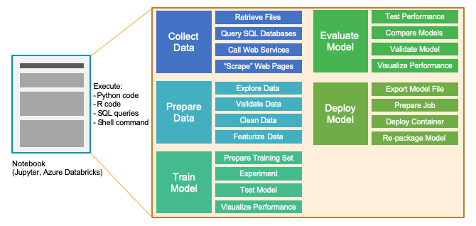
Notebooks are made up of one or more cells that allow for the execution of the code snippets or commands within those cells. They store commands and the results of running those commands. In this diagram, you can see that we can use a notebook environment to perform the five primary stages of model development:
Basic Modeling
Experiments:
An experiment is a general context for handling runs. Think about it as a folder that organizes the artifacts used in your Model Training process. Once you have an experiment, you can create runs within that experiment.
Runs:
A run is a single execution of a training script to train a model. It contains all artifacts associated with the training process, like output files, metrics, logs, and a snapshot of the directory that contains your scripts.
Run Configurations: a set of instructions that defines how a script should be run in a specified compute target. A run configuration can be persisted into a file inside the directory that contains the training script, or it can be constructed as an in-memory object and used to submit a run.
It includes a wide set of behavior definitions such as whether to use existing Python environments or to use a Conda environment that’s built from a specification. A run can have zero or more chart runs.
Models:
A run is used to produce a model. Essentially, a model is a piece of code that takes input and produces output. To get a model, we start with a more general algorithm. By combining this algorithm with the training data — as well as by tuning the hyperparameters — we produce a more specific function that is optimized for the particular task we need to do. Put concisely:
Model = algorithm + data + hyperparameters
Model Registry:
A registered model is a logical container for one or more files that make up the model. Once we have a trained model, we can turn to the model registry, which keeps track of all models in an Azure Machine Learning workspace. Note that models are either produced by a Run or originate from outside of Azure Machine Learning (and are made available via model registration).
Advanced Modeling
Machine Learning Pipelines:
As the process of building your models becomes more complex, it becomes more important to get a handle on the steps to prepare your data and train your models in an organized way. In these scenarios, there can be many steps involved in the end-to-end process, including:
Data ingestion
Data preparation
Model building & training
Model deployment.
These steps are organized into machine learning pipelines.
You use machine-learning pipelines to create and manage workflows that stitch together the machine-learning phases. There are cyclical and iterative in nature and facilitate continuous improvement of model performance, model deployment, and making inferences over the best performing model to date.
Machine-learning pipelines are made up of distinct steps:
Machine Learning Pipelines are modular which makes the steps usable and run without rerun in subsequent steps if the output of the steps has been changed.
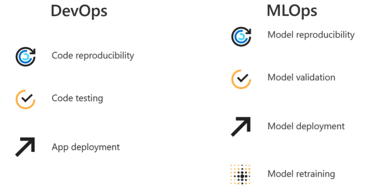
Instead of manual processes, we want to develop processes that use automated builds and deployments. The general term for this approach is DevOps; when applied to machine learning, we refer to the automation of machine learning pipelines as MLOps.
Important aspects of MLOps:
Automating the end-to-end ML life cycle,
Monitoring ML solutions for both generic and ML specific operational issues
Capturing all data that is necessary for full traceability in the ML life cycle
Operationalizing Models
Operationalization refers to the deployment of a machine learning model after it has been trained and evaluated to the point where it is ready to be used outside of a development or test environment.
Typical Model Deployment:
Get the model file (any file format)
Create a scoring script (.py)
Optionally create a schema file describing the web service input (.json)
Create a real-time scoring web service
Call the web service from applications
Repeat the process each time the model is re-trained
Real-time Inferencing:
The model training process can be very compute-intensive, with training times that can potentially span across many hours, days, or even weeks. A trained model, on the other hand, is used to make decisions on new data quickly. In other words, it infers things about new data it is given based on its training. Making these decisions on new data on-demand is called Real-time Inferencing.
Batch Inferencing:
Unlike real-time inferencing, which makes predictions on data as it is received, Batch Inferencing is run on large quantities (batches) of existing data. Typically, batch inferencing is run on a recurring schedule against data stored in a database or other data store. The resulting predictions are then written to a data store for later use by applications, data scientists, developers, or end-users.
Batch scoring is used typically when historical time-based data is to be considered that is as long as possible and the value has to be predicted at a certain level of granularity. It typically involves latency requirements of hours or days so it doesn’t require using train models deployed to restful web services, as is done for real-time inference. Use Batch Inferencing when:
No need for real-time
Inferencing results can be persisted
Post-processing or analysis of the predictions is needed
Inferencing is complex
Due to the scheduled nature of batch inferencing, predictions are not usually available for new data. However, in many common real-world scenarios, predictions are needed on both newly arriving and existing historical data. This is where Lambda Architecture comes in.
The gist of the Lambda architecture is that ingested data is processed at two different speeds. A Hot path that tries to make predictions against the data in real-time, and a cold path that makes predictions in a batch fashion, which might take days to complete.
Programmatically Accessing Managed Services
Data scientists and AI developers use Azure Machine Learning SDK for Python to build and run machine learning workflows with the Azure Machine Learning service. You can interact with the service in any Python environment, including Jupyter Notebooks, Visual Studio Code, and your favorite Python IDE.
Key areas of the SDK include:
Manage datasets
Organize and monitor experiments
Model training
Automated Machine Learning
Model deployment
Azure Machine Learning service supports many of the popular open-source machine learning and deep learning Python packages that we discussed earlier in the course, such as:
Scikit-learn
Tensorflow
PyTorch
Keras
Lesson Summary
In this lesson, you’ve learned about managed services for Machine Learning and how these services are used to enhance Machine Learning processes.
First, you learned about various types of computing resources made available through managed services, including:
Training compute
Inferencing compute
Notebook environments
Next, you studied the main concepts involved in the modeling process, including:
Basic modeling
How parts of the modeling process interact when used together
More advanced aspects of the modeling process, like automation via pipelines and end-to-end integrated processes (also known as DevOps for Machine Learning or simply, MLOps)
How to move the results of your modeling work to production environments and make them operational
Finally, you were introduced to the world of programming the managed services via the Azure Machine Learning SDK for Python.
Unselfie: Translating Selfies to Neutral-pose Portraits in the Wild; How to Evaluate the Performance of Your Machine Learning Model; Deep Learning Most Important Ideas – an excellent review
Join this exclusive Reuters Events webinar: Technology enabled customer-centric innovation with Travelers, Wells Fargo and Henkel, on Aug 20 @ 11:00 ET, and learn how to marry both concepts to delight your consumers with data driven customer-centric innovation!
This article uses PyCaret 2.0, an open source, low-code machine learning library in Python to develop a simple AutoML solution and deploy it as a Docker container using GitHub actions.