365 Data Science

Roadmap to Data Science

In this article, I will give you a complete road map on how to become a Data Scientist with skills like Machine Learning, Deep Learning and Artificial Intelligence.

So you probably are thinking that you need a Masters Degree or PhD from a great university to become a Data Scientist. Somehow it’s true that having a Masters or PhD in this background from a very top university will open doors for us in the field of Data Science and Machine Learning.

But you really don’t need any degree in order to become a Data Scientist, Let me explain how to do it.

How to Become a Data Scientist

There are 5 steps to become a Data Scientist, they are:

1. Learn Python

Python is a Great Language for Data Science, Now there will be some people who will say, to learn R or Matlab instead of python. Just don’t listen to them. Yet one day you might need to learn R and Matlab.

But to begin with, Python is the best choice for me, because the support of external libraries for Data Science and Machine Learning is best and easy in python.

2. Learn Mathematics(Linear Algebra and Statistics)

Data Science is all about applying maths to data. If you don’t know about maths, you will face difficulties with data science. You can start learning Mathematics for Data Science using Numerical Python and Statistics.

3. Learn Python Libraries

The Python Libraries are absolutely fantastic. If you don’t know what a library is, It’s basically something that you can add on to python, that gives python a lot more functionality.

There are some great Libraries for Data Science, you are required to learn:

1. Numpy (for linear algebra)
2. Pandas (for statistics and data manipulation)
3. Matplotlib (for data visualization)
4. Scikit-Learn (for Machine Learning)
5. Learn Every Topic of Data Science

4. Start working on projects

After learning all these libraries you can start working on your own projects. You can get more than 20 projects here at — Data Science and Machine Learning Projects, or otherwise, you can research on the Internet to download the data sets for your practice.

You can download the data sets from https://catalog.data.gov/dataset, and if you want to work on projects related to Finance then https://in.finance.yahoo.com/ would be best for you.

5. Register yourself with Github

The last step is to register yourself at Github, here you can share your projects with everyone in the world.

The idea is to create a good portfolio of your projects at Github, so that people may know about you that what you do and what is your level with Programming.

Try to upload at least one project every month on Github, so that when employers will ask you for your contribution to any project, you can impress him with your skills.

Don’t forget to give us your ? !

---

Roadmap to Data Scientist was originally published in Becoming Human: Artificial Intelligence Magazine on Medium, where people are continuing the conversation by highlighting and responding to this story.

Via https://becominghuman.ai/roadmap-to-data-scientist-b1dcb17896e7?source=rss—-5e5bef33608a—4

Welcome to My Week in AI! Each week this blog will have the following parts:

• What I have done this week in AI
• An overview of an exciting and emerging piece of AI research

Progress Update

Unearthing new tools

This week I came across two tools that I wanted to share, as I think they would be useful additions to a data science toolkit. First is Elasticsearch, an open-source search and analytics library for a range of different data types including textual, numerical and geospatial. It processes data quickly and is very scalable, and because of this has a number of use cases such as log analytics, geospatial data analysis and application search. Second is Streamlit, an easy way to build interactive Python apps for machine learning. The app updates as soon as you make changes to the code, so you can view your changes in almost real time. Overall, it is a powerful tool for Data Scientists and Machine Learning Engineers who want to visualize data and display their results in an aesthetically pleasing and interactive manner.

Learning new skills

From my personal experience and from talking to colleagues, I believe that there is often a knowledge gap for people starting out as Machine Learning Engineers. We often know how to deploy models (for former Software Engineers), or how to train models (for former Data Scientists), but not many of us have knowledge of both. In my research, I’ve found that many good and free resources are available for learning about training models, but I have not been able to find the same for deploying models. That is why I was so excited when a friend of mine recommended the Full Stack Deep Learning course, a free two-day online bootcamp in shipping deep learning projects. The course includes a project in which you have to deploy a deep learning system into production, and this hands-on experience is invaluable. This is definitely a course that I hope to complete over the next couple of weeks.

Emerging Research

Efficient graph similarity search

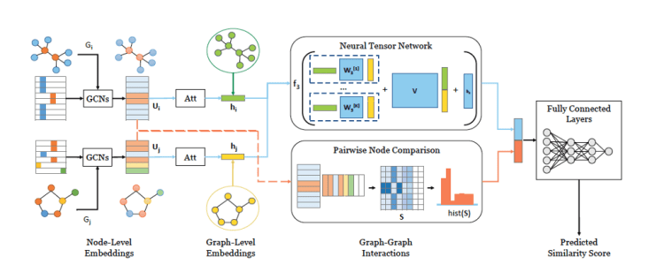
This week’s research is about graph similarity search, a task often associated with identifying similar chemical molecules. Bai et al. present a new method of graph similarity search in: ‘SimGNN: A Neural Network Approach to Fast Graph Similarity Computation.’ They propose a fast and accurate method of determining the similarity between two graphs by turning this task into a learning problem, using a neural network-based function that is trained to compute the similarity score between two graphs.¹

Their method proceeds in the following manner:

1. The nodes are encoded based on the features and structural properties around them.

2. A learnable embedding function generates an embedding vector for each graph, providing a summary of the graph information using an attention mechanism.

3. In the interaction stage, the node-level and graph-level embeddings of two graphs are compared respectively and interaction scores are computed.

4. The two sets of interaction scores are passed into a fully connected layer to obtain a final similarity score.

For the learnable embedding function, the researchers used a Graph Convolutional Network as these types of networks can be configured to be representation-invariant and inductive — two important properties for this task.

This method was consistently the most accurate for graph similarity search on benchmark datasets, when compared with other state-of-the-art methods such as Beam and AttDegree. The authors also found that SimGNN was 46 times faster than Beam search on large graphs, another key performance marker in its favor. The total time taken included the time for training; if a pre-trained version of SimGNN was used, and then fine-tuned to a specific dataset, then this method would be even faster.

The researchers highlighted the potential applications of this method in bioinformatics, social network analysis, recommender systems and more, and I believe this is an exciting new method in the area of graph deep learning.

Next week I will be presenting more of my work in AI and discussing research on the use of AI in drug discovery. Thanks for reading and I appreciate any comments/feedback/questions.

References

[1] Bai, Y., Ding, H., Bian, S., Chen, T., Sun, Y., & Wang, W. (2019). SimGNN: A Neural Network Approach to Fast Graph Similarity Computation. Proceedings of the Twelfth ACM International Conference on Web Search and Data Mining. doi:10.1145/3289600.3290967

Don’t forget to give us your ? !

---

My Week in AI: Part 8 was originally published in Becoming Human: Artificial Intelligence Magazine on Medium, where people are continuing the conversation by highlighting and responding to this story.

Via https://becominghuman.ai/my-week-in-ai-part-8-ce0e0d1d6eff?source=rss—-5e5bef33608a—4

I have a machine learning joke, but it is not performing as well on a new audience. We bring you a selection of the nerdy self-referential computer jokes that were popular on the web recently.

Originally from KDnuggets https://ift.tt/2PhHa7M

Combining different data sources is a time suck! d6tjoin is a python library that lets you join pandas dataframes quickly and efficiently.

Originally from KDnuggets https://ift.tt/3fcDDSt

Concept of Regression Analysis for Time Series Data and Detecting Autocorrelation using The Durbin-Watson Test

Before start my main topic, I would like to introduce you about Regression Analysis and Time Series Data in shortly.

What is Regression Analysis?

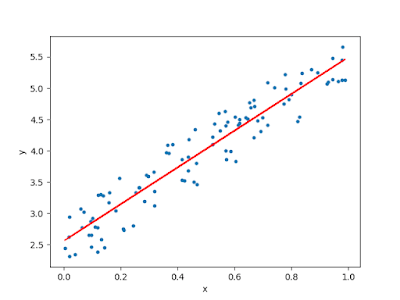
Regression analysis is a statistical techniques in machine learning, which is most popular and frequently used techniques. This techniques is useful for investigating and modelling the relationship between dependent feature/variable (y) and one or more independent features/variables (x)

Time Series Data:

In simple word, time series data is data such that its points are recorded at time sequence. In other word, data is collected at different point in time.

Example : Annual Expenditures of particular person.

Hope, you may have understood what is regression analysis and time series data. Let’s come to the point.

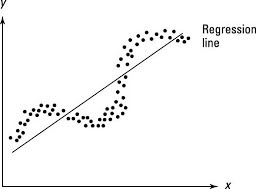
Many applications of regression analysis involve both independent/predictor and dependent/response variables that are time series, that mean, the variables are recorded at time sequence. The assumption of uncorrelated or independent errors that is typically made for regression data that is not time-dependent is usually not appropriate for time series data. The error in time series data represent autocorrelated structure. Autocorrelation, also known as serial correlation, tell that the error are correlated with different time period itself.

Sources of autocorrelation in time series regression data :

There are many sources of auto-correlation in time series regression data. In many cases, the cause of autocorrelation is the failure of the analyst to include one or more important predictor variable in the model.

Ex : Suppose that we wish to regress the sales of a product in a particular region of the country against the annual advertising expenditures for that product.

In above example, the growth in the population in that region over the period of time used in the study will also influence the product sale. Failure to include the population size may cause the errors in the model to be positively autocorrelated, because if the per-capita demand for the product is either constant or increasing with time, population size is positively correlated with product sales.

The presence of autocorrelation in the errors has several effect on the ordinary least-squares regression procedure.

1. Regression coefficient are still unbiased, but they are no longer minimum- variance estimates.
2. When the errors are positively autocorrelated, the residual mean square may seriously underestimate the error variance.
3. Confidence intervals, prediction intervals, and tests of hypotheses base on t and F distributions are, strictly speaking, no longer exact procedures.

Dealing with the autocorrelation:

We can deal with autocorrelation using three approaches. If autocorrelation present due to failure of to include one or more predictors and if analyst can be identified and include those predictor in the model, then observed autocorrelation should disappear.

As another option to dealing with the problem of autocorrelation, the weighted least squares or generalised least squared method could be used if there were sufficient knowledge of the autocorrelation structures. If these approaches cannot be used then the analyst must turn to a model that specifically include the autocorrelation structure. These models usually require special parameter estimation techniques. How can we identify autocorrelaion present or not in your data? This most very common question arise for every analyst. So that is what, I am going to discuss about how we can detect autocorrelation using statistical techniques with example.

Trending AI Articles:

1. Natural Language Generation:
The Commercial State of the Art in 2020

2. This Entire Article Was Written by Open AI’s GPT2

3. Learning To Classify Images Without Labels

4. Becoming a Data Scientist, Data Analyst, Financial Analyst and Research Analyst

Detecting autocorrelation:

For the detection of autocorrelation, residual plots can be useful. Draw the plot of residuals versus time for meaningful and useful visualisation.

There are two possibility while detecting autocorrelation.

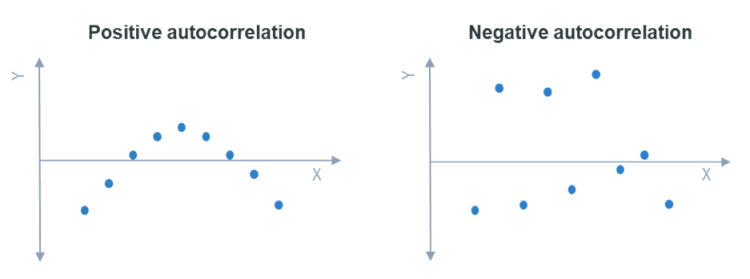
Positive autocorrelation : Positive autocorrelation is indicated by a cyclical residual plot over time. The correlation is positive between observation which were recorded in time sequence.

Negative autocorrelation : Negative autocorrelation is indicated by alternating pattern where the residual cross time axis more frequently than if they were distributed randomly. The correlation is negative between observation which were recorded in time sequence.

See the below figure, which is visualisation of autocorrelation. Figure is showing the relation between residuals(Y-axis) and time(X-axis).

The Durbin-Watson Test:

Various statistical tests can be used to detect the presence of autocorrelation. The test developed by Durbin and Watson (1950, 1951, 1971) is a very widely used procedure. This test for first order autocorrelation — i.e. assume that the errors in the regression model are generated by a first-order autoregressive process observed at equally spaced time period.

For uncorrelated errors lag one sample autocorrelation coefficient equal to 0 (at least approximately) so the value of Durbin-Watson statistic should be approximately 2. Statistical testing is necessary to determine just how far away from 2 the statistic must fall in order for us to conclude that the assumption of uncorrelated errors is violated. The decision procedure is as follows.

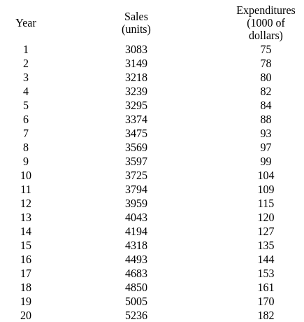
Example: A company wants to use a regression model to related annual regional advertising expenses to annual regional concentrate sale for a soft drink company. Table 1 presents 20 years of these data. we will initially assume that a linear relationship is appropriate and fit simple linear regression by ordinary least squares.

Fitting a simple linear regression model by using python:

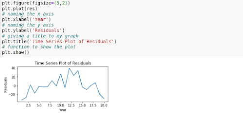
The plot of residuals versus time, shown in below figure.

Residuals plot has a pattern indicative of potential autocorrelation; there is a definite upward trend in the plot.

Hypothesis:

Null hypothesis : There is no autocorrelation present in errors of model Alternative hypothesis : There is positive autocorrelation present in errors of model

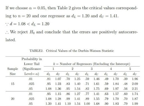
Result:

conclusion:

Endnote : A significant value of the Durbin-Watson statistic or a suspicious residual plot indicates a potential problem with autocorrelated model errors. This could be the result of an actual time dependence in the error or and ‘artificial’ time dependence caused by the omission of one or more important predictor variable. If the apparent autocorrelation result from missing predictors and if these missing predictors can be identified and incorporated into the model, the autocorrelation problem may be eliminated. If autocorrelation cannot removed by one or more new predictor, it is necessary to take explicit account of the autocorrelative structure in the model and use an appropriate parameter estimation method. A very good and widely used approach is the procedure devised by Cochrane and Orcutt(1949).

Montgomery, D. C., Peck, E. A. and Vining, G. G. (2001). Introduction to Linear Regression Analysis. 3rd Edition, New York, New York: John Wiley & Sons.

Don’t forget to give us your ? !

---

Concept of Regression Analysis for Time Series Data and Detecting Autocorrelation using The… was originally published in Becoming Human: Artificial Intelligence Magazine on Medium, where people are continuing the conversation by highlighting and responding to this story.

Via https://becominghuman.ai/concept-of-regression-analysis-for-time-series-data-and-detecting-autocorrelation-using-the-85bde275b797?source=rss—-5e5bef33608a—4

In this blog, I’m going to use Diabetes dataset which I got from Kaggle. I’ll be showing you how to analyse the data and apply different Machine Learning Classification Models.

So I have used 4 different ML models for predicting Diabetes.

1. RandomForest

Random forests or random decision forests are an ensemble learning method for classification, regression and other tasks that operate by constructing a multitude of decision trees at training time and outputting the class that is the mode of the classes or mean prediction of the individual trees.

2. SVC

SVC is a nonparametric clustering algorithm that does not make any assumption on the number or shape of the clusters in the data. In our experience, it works best for low-dimensional data, so if your data is high-dimensional, a preprocessing step, e.g. using principal component analysis, is usually required.

3. KNN

In pattern recognition, the k-nearest neighbour’s algorithm (k-NN) is a non-parametric method proposed by Thomas Cover used for classification and regression. In both cases, the input consists of the k closest training examples in the feature space. The output depends on whether k-NN is used for classification or regression:

4. Decision Tree

Decision Tree algorithm belongs to the family of supervised learning algorithms. … The goal of using a Decision Tree is to create a training model that can use to predict the class or value of the target variable by learning simple decision rules inferred from prior data(training data).

So now let’s jump in coding

Import the necessary libraries.

import pandas as pd
import matplotlib.pyplot as plt
import numpy as np
import seaborn as sns
import matplotlib.pyplot as plt
%matplotlib inline

Load Dataset

data = pd.read_csv(“Datasets/pima-data.csv”)

Understand the dataset

data.head()

Trending AI Articles:

1. Natural Language Generation:
The Commercial State of the Art in 2020

2. This Entire Article Was Written by Open AI’s GPT2

3. Learning To Classify Images Without Labels

4. Becoming a Data Scientist, Data Analyst, Financial Analyst and Research Analyst

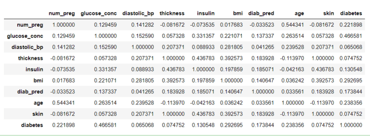
Getting co-relations of all the features

data.corr()

Change the diabetes feature in Boolean form

diabetes_map = {True: 1, False: 0}
data[‘diabetes’] = data[‘diabetes’].map(diabetes_map)

data.head()

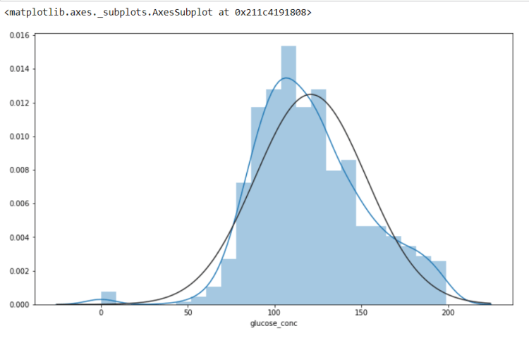
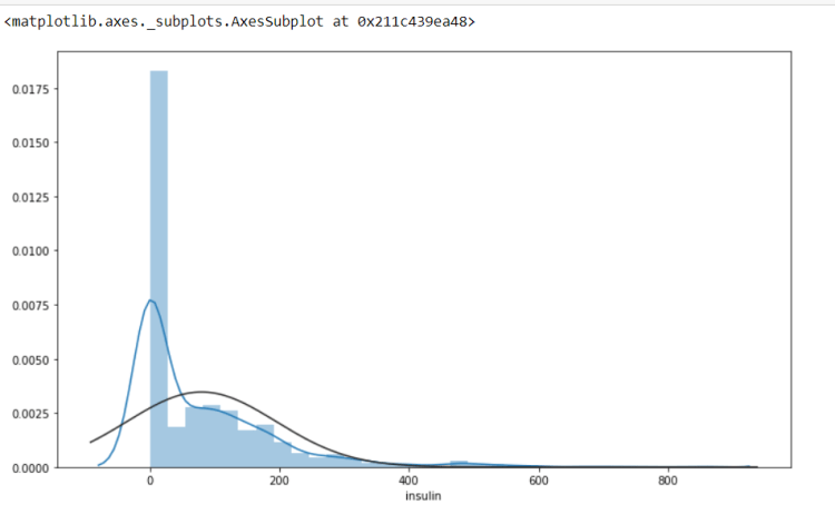
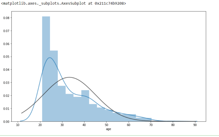
Analysing The Data

plt.figure(figsize=(12,7))
sns.distplot(data[‘glucose_conc’],kde=True,fit=norm)

plt.figure(figsize=(12,7))
sns.distplot(data[‘insulin’],kde=True,fit=norm)

plt.figure(figsize=(12,7))
sns.distplot(data[‘age’],kde=True, fit=norm)

Split the dataset into training and testing

from sklearn.model_selection import train_test_split
feature_columns = ['num_preg', 'glucose_conc', 'diastolic_bp', 'insulin', 'bmi', 'diab_pred', 'age', 'skin']
predicted_class = ['diabetes']
X = data[feature_columns].values
y = data[predicted_class].values
X_train, X_test, y_train, y_test = train_test_split(X, y, test_size = 0.30, random_state=10)

Apply SimpleImputer for missing data

from sklearn.impute import SimpleImputer
fill_values = SimpleImputer(missing_values=0, strategy=”mean”)
X_train = fill_values.fit_transform(X_train)
X_test = fill_values.fit_transform(X_test)

Applying different Classification Algorithms

1. RandomForest

# RandomForest Algorithm
from sklearn.ensemble import RandomForestClassifier
random_forest_model = RandomForestClassifier(random_state=10)
random_forest_model.fit(X_train, y_train.ravel())
randomforest_prediction = random_forest_model.predict(X_test)

2. SVC

# SVC Algorithm
from sklearn.svm import SVC
svc_model = SVC(kernel = ‘rbf’, random_state = 0)
svc_model.fit(X_train, y_train.ravel())
svc_prediction = svc_model.predict(X_test)

3. KNN

# KNeighborsClassifier Algorithm
from sklearn.neighbors import KNeighborsClassifier
knn_classifier = KNeighborsClassifier(n_neighbors = 5, metric = ‘minkowski’, p = 2)
knn_classifier.fit(X_train, y_train.ravel())
knn_prediction = knn_classifier.predict(X_test)

4. Decision Tree

# Decision Tree Algorithm
from sklearn.tree import DecisionTreeClassifier
decisiontree_classifier = DecisionTreeClassifier(criterion = ‘entropy’, random_state = 0)
decisiontree_classifier.fit(X_train, y_train.ravel())
decisiontree_prediction = decisiontree_classifier.predict(X_test)

Analysing the accuracy of all the 4 models

from sklearn import metrics

print(“Accuracy RandomForest = {0:.3f}”.format(metrics.accuracy_score(y_test, randomforest_prediction)))
print(“Accuracy SVC = {0:.3f}”.format(metrics.accuracy_score(y_test, svc_prediction)))
print(“Accuracy KNN = {0:.3f}”.format(metrics.accuracy_score(y_test, knn_prediction)))
print(“Accuracy Decision Tree = {0:.3f}”.format(metrics.accuracy_score(y_test, decisiontree_prediction)))

You can find the complete source code along with dataset here.

So from the above accuracy RandomForest model is best for this dataset. As it provides 73.6% accuracy.

Don’t forget to give us your ? !

---

Machine Learning Models for Detecting Diabetes. was originally published in Becoming Human: Artificial Intelligence Magazine on Medium, where people are continuing the conversation by highlighting and responding to this story.

Via https://becominghuman.ai/machine-learning-models-for-detecting-diabetes-c85b55684aa2?source=rss—-5e5bef33608a—4

Welcome to My Week in AI! Each week this blog will have the following parts:

• What I have done this week in AI
• An overview of an exciting and emerging piece of AI research

Progress Update

Testing for machine-learning code

In my work this week at Blueprint Power, I spent a lot of time developing time series forecasting models. It is important that these models are robust from a software engineering perspective; a part of that is unit testing, which is not an easy task for machine-learning code. There are several reasons why this is difficult, including:

· A bug can be confused with poor model architecture or hyperparameters

· We don’t always know what the expected outputs should be

· Interpretability is difficult with neural networks, so it can be hard to pinpoint where an error occurs

Unit testing is especially challenging when using a deep learning framework, such as PyTorch, where much of the computation is done for you by the framework. That is why I was excited to come across torchtest, a library that directly tests for common bugs in a PyTorch deep learning model. The library tests for four bugs:

1. Variables that are supposed to change during training change, and the variables that are not supposed to change don’t change

2. Output range of the logits is unreasonable (as defined by the user)

3. There are no NaN outputs

4. There are no inf outputs

This library makes implementing unit tests for PyTorch code much easier. Although it is limited because it does not allow you to reach 100% test coverage, it is a start, and should make model development a less frustrating process as I will be able to catch and identify bugs more quickly.

Trending AI Articles:

1. Natural Language Generation:
The Commercial State of the Art in 2020

2. This Entire Article Was Written by Open AI’s GPT2

3. Learning To Classify Images Without Labels

4. Becoming a Data Scientist, Data Analyst, Financial Analyst and Research Analyst

Emerging Research

Identifying unknown samples at test time

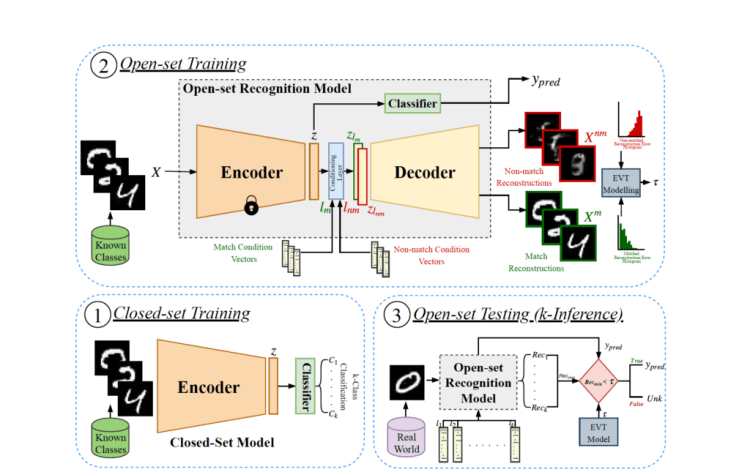
As I mentioned in my last post , this week I’m presenting research on the use of autoencoders in computer vision, specifically in open-set recognition. ‘C2AE: Class Conditioned Auto-Encoder for Open-set Recognition’ by Oza and Patel presents a new, open-set recognition method based on class-conditioned auto-encoders that divides the open-set problem into sub-tasks. The open-set problem occurs when a classification algorithm sees an unknown class sample during inference and is forced to classify this sample as a class from the closed-set used in training. This negatively impacts the performance of such a classifier. In this scenario, we would instead like to classify that sample as ‘unknown’.

The proposed method splits the open-set recognition task into two sub-tasks: closed-set classification and open-set identification. The closed-set classification sub-task is trained using the commonly used encoder and classifier architecture. The open-set identification sub-task is split into two further components: conditional decoder training and Extreme Value Theory modeling of the reconstruction errors. For conditional decoder training, the encoder is used to extract the latent vectors and then the decoder is trained to perfectly reconstruct the original input when given the label condition vector matching the class of the input. In this research, the decoder was also trained to badly reconstruct the original input when given the label condition vector that does not match the class of the input. The authors showed that this non-match training was representative of an open-set situation at inference. Next, Extreme Value Theory modeling was used to model the reconstruction errors and to classify a sample as known/unknown.

The researchers saw significant improvement when evaluating this method against previous state-of-the-art techniques,, and this approach also achieves a near 0.2 increase in F-score performance on the Labeled Faces in the Wild dataset when compared with the next best method.

I found this work fascinating as it provides a strong and interpretable solution to the problem of samples of unknown classes during inference. Beyond naively setting a threshold on the Softmax values to classify low probability samples as ‘unknown’, I had not previously considered any solutions to this problem. I also thought this was a noteworthy use of autoencoders, which are becoming more and more prevalent in deep learning literature.

Next week I will be presenting more of my work in AI, and once again, sharing a piece of exciting research. Thanks for reading and I appreciate any comments/feedback/questions.

References

[1] Oza, P., & Patel, V. M. (2019). C2AE: Class Conditioned Auto-Encoder for Open-Set Recognition. 2019 IEEE/CVF Conference on Computer Vision and Pattern Recognition (CVPR). doi:10.1109/cvpr.2019.00241

Don’t forget to give us your ? !

---

My Week in AI: Part 7 was originally published in Becoming Human: Artificial Intelligence Magazine on Medium, where people are continuing the conversation by highlighting and responding to this story.

Via https://becominghuman.ai/my-week-in-ai-part-7-15d86038dd7a?source=rss—-5e5bef33608a—4

The fact that R-squared shouldn’t be used for deciding if you have an adequate model is counter-intuitive and is rarely explained clearly. This demonstration overviews how R-squared goodness-of-fit works in regression analysis and correlations, while showing why it is not a measure of statistical adequacy, so should not suggest anything about future predictive performance.

Originally from KDnuggets https://ift.tt/3fkohvg

Scaling Machine Learning models is hard and expensive. We will shortly introduce the Google Cloud service Dataflow, and how it can be used to run predictions on millions of images in a serverless way.

Originally from KDnuggets https://ift.tt/2D8QDM7

Check out this list of awesome, free machine learning and artificial intelligence courses with video lectures.

Originally from KDnuggets https://ift.tt/33bsI9d