365 Data Science

The new tools shows the potential of data visualizations for understanding features in a neural network.

Originally from KDnuggets https://ift.tt/34IwzcN

Enterprises are struggling to launch machine learning models that encapsulate the optimization of business processes. These are now the essential components of data-driven applications and AI services that can improve legacy rule-based business processes, increase productivity, and deliver results. In the current state of the industry, many companies are turning to off-the-shelf platforms to increase expectations for success in applying machine learning.

Originally from KDnuggets https://ift.tt/2xAJbGD

In the first part of this series we discussed the concept of a neural network, as well as the math describing a single neuron. There are however many neurons in a single layer and many layers in the whole network, so we need to come up with a general equation describing a neural network.

1: Passing the information through — Feed Forward

Single neuron

The first thing our network needs to do is pass information forward through the layers. We already know how to do this for a single neuron:

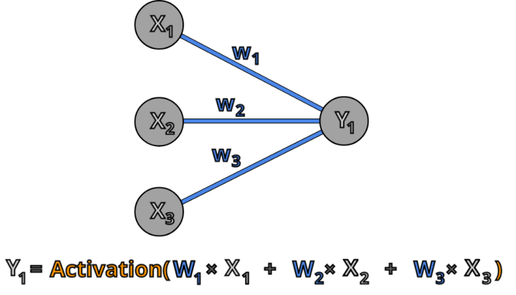
Output of the neuron is the activation function of a weighted sum of the neuron’s input

2 neurons

Now we can apply the same logic when we have 2 neurons in the second layer.

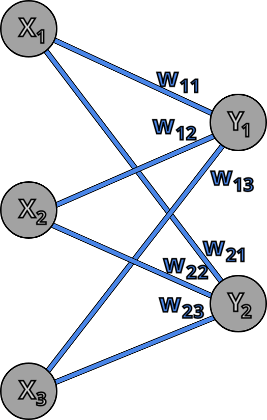
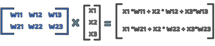
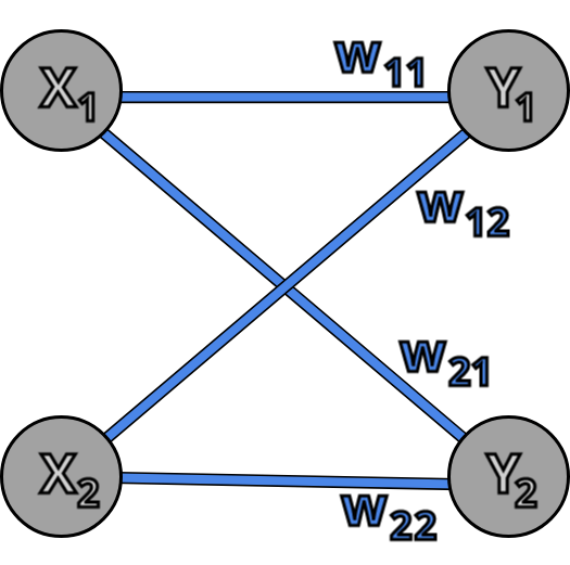
In this example every neuron of the first layer is connected to each neuron of the second layer, this type of network is called fully connected network. Neuron Y1 is connected to neurons X1 and X2 with weights W11 and W12 and neuron Y2 is connected to neurons X1 and X2 with weights W21 and W22. In this notation the first index of the of the weight indicates the output neuron and the second index indicates the input neuron, so for example W12 is weight on connection from X2 to Y1. Now we can write the equations for Y1 and Y2:

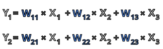
Now this equation can be expressed using matrix multiplication.

If you are new to matrix multiplication and linear algebra and this makes you confused i highly recommend 3blue1brown linear algebra series.

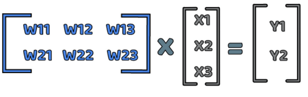
Now we can write output of first neuron as Y1 and output of second neuron as Y2. This gives us the following equation:

Whole layer

From this we can abstract the general rule for the output of the layer:

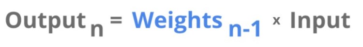
Now in this equation all variables are matrices and the multiplication sign represents matrix multiplication.

Usage of matrix in the equation allows us to write it in a simple form and makes it true for any number of the input and neurons in the output.

In programming neural networks we also use matrix multiplication as this allows us to make the computing parallel and use efficient hardware for it, like graphic cards.

Now we have equation for a single layer but nothing stops us from taking output of this layer and using it as an input to the next layer. This gives us the generic equation describing the output of each layer of neural network. One more thing, we need to add, is activation function, I will explain why we need activation functions in the next part of the series, for now you can think about as a way to scale the output, so it doesn’t become too large or too insignificant.

With this equation, we can propagate the information through as many layers of the neural network as we want. But without any learning, neural network is just a set of random matrix multiplications that doesn’t mean anything.

So how to teach our neural network? Firstly we need to calculate the error of the neural network and think how to pass this error to all the layers.

2 : Passing the error — Back-propagation

To understand the error propagation algorithm we have to go back to an example with 2 neurons in the first layer and 1 neuron in the second layer.

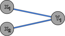
Let’s assume the Y layer is the output layer of the network and Y1 neuron should return some value. Now this value can be different from the expected value by quite a bit, so there is some error on the Y1 neuron. We can think of this error as the difference between the returned value and the expected value. We know the error on Y1 but we need to pass this error to the lower layers of the network because we want all the layers to learn, not only Y layer. So how to pass this error to X1 and X2? Well, a naive approach would be to split the Y1 error evenly, since there are 2 neurons in the X layer, we could say both X1 and X2 error is equal to Y1 error devised by 2.

There is however a major problem with this approach — the neurons have different weights connected to them. If the weight connected to the X1 neuron is much larger than the weight connected to the X2 neuron the the error on Y1 is much more influenced by X1 since Y1 = ( X1 * W11 + X2 * X12). So if W11 is larger than W12 we should pass more of the Y1 error to the X1 neuron since this is the neuron that contributes to it.

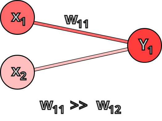
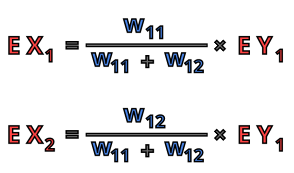
Now that we have observed it we can update our algorithm not to split the error evenly but to split it according to the ration of the input neuron weight to all the weights coming to the output neuron.

Now we can go one step further and analyze the example where there are more than one neuron in the output layer.

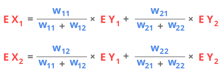
In this example we see that e.g. neuron X1 contributes not only to the error of Y1 but also to the error of Y2 and this error is still proportional to its weights. So, in the equation describing error of X1, we needto have both error of Y1 multiplied by the ratio of the weights and error of Y2 multiplied by the ratio of the weights coming to Y2.

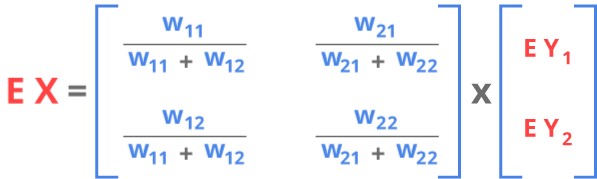
This equation can also be written in the form of matrix multiplication.

Now there is one more trick we can do to make this quotation simpler without losing a lot of relevant information. The denominator of the weight ratio, acts as a normalizing factor, so we don’t care that much about it, partially because the final equation we will have other means of regulating the learning of neural network.

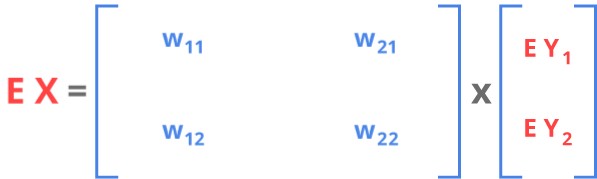
This is also one more observation we can make. We can see that the matrix with weight in this equation is quite similar to the matrix form the feed forward algorithm. The difference is the rows and columns are switched. In algebra we call this transposition of the matrix.

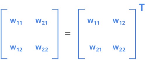
Since there is no need to use 2 different variables, we can just use the same variable from feed forward algorithm. This gives us the general equation of the back-propagation algorithm

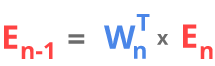
Note that in the feed-forward algorithm we were going form the first layer to the last but in the back-propagation we are going form the last layer of the network to the first one since to calculate the error in a given layer we need information about error in the next layer.

Trending AI Articles:

1. How I used machine learning as inspiration for physical paintings

2. MS or Startup Job — Which way to go to build a career in Deep Learning?

3. TOP 100 medium articles related with Artificial Intelligence

4. Artificial Intelligence Conference

Now that we know how to pass the information forward and pass the error backward we can use the error at each layer to update the weight.

3 : Updating the weights

Now that we know what errors does out neural network make at each layer we can finally start teaching our network to find the best solution to the problem.

But what is the best solution?

The error informs us about how wrong our solutions is, so naturally the best solution would be the one where the error function is minimal.

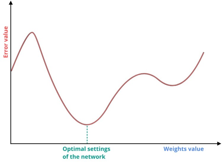
Error function depends on the weights of the network, so we want to find such weights values that result in the global minimum in the error function. Note that this picture is just for the visualization purpose. In real life applications we have more than 1 weight, so the error function is high-dimensional function.

But how do we find the minimum of this function? A simple idea here is to start with random weights, calculate the error function for those weights and then check the slope of this function to go downhill.

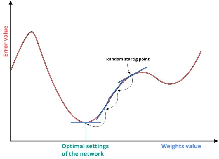
But how do we get to know the slope of the function?

We can use linear algebra once again and leverage the fact that derivative of a function at given point is equal to the slope a function at this point. We can write this derivative in the following way:

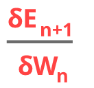
Where E is our error function and W represents the weights. This notation informs us that we want to find the derivative of the error function with respect to weight. We use n+1 in with the error, since in our notation output of neural network after the weights Wn is On+1.

We can then use this derivative to update the weight:

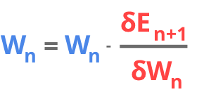
This represents the “going downhill” each learning iteration (epoch) we update the weight according to the slope of the derivative of the error function.

There is one more thing we need before presenting the final equation and that is learning-rate. Learning-rate regulates how big steps are we taking during going downhill.

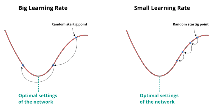
As you can see with bigger learning rate, we take bigger steps. This means we can get to the optimum of the function quicker but there is also a grater chance we will miss it.

With the smaller learning rate we take smaller steps, which results in need for more epochs to reach the minimum of the function but there is a smaller chance we miss it.

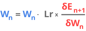
That’s why in practice we often use learning rate that is dependent of the previous steps eg. if there is a strong trend of going in one direction, we can take bigger steps (larger learning rate), but if the direction keeps changing, we should take smaller steps (smaller learning rate) to search for the minimum better. In our example however, we are going to take the simple approach and use fixed learning rate value. This gives us the following equation.

Learning rate (Lr) is a number in rage 0 — 1. The smaller it is, the lesser the change to the weights. If learning is close to 1. we use full value of the derivative to update the weights and if it is close to 0, we only use a small part of it. This means that learning rate, as the name suggests, regulates how much the network “learns” in a single iteration.

Updating the weights was the final equation we needed in our neural network. It is the equations that is responsible for the actual learning of the network and for teaching it to give meaningful output instead of random values.

Putting it all together

Don’t forget to give us your ? !

---

Understanding neural networks 2: The math of neural networks in 3 equations was originally published in Becoming Human: Artificial Intelligence Magazine on Medium, where people are continuing the conversation by highlighting and responding to this story.

Via https://becominghuman.ai/understanding-neural-networks-2-the-math-of-neural-networks-in-3-equations-6085fd3f09df?source=rss—-5e5bef33608a—4

Creating an API with Heroku is Simple one , you can do it very quickly.

Now we are going to create an API for sentiment analysis , you can also alternate the code any machine learning model

I created a folder name as sentiment_analysis

At minimum level your file should contain these .

we will get those one by one

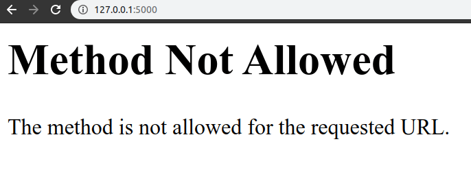
this is an simple flask app for giving the result the text is positive or negative or neutral , just save this and run the app.py

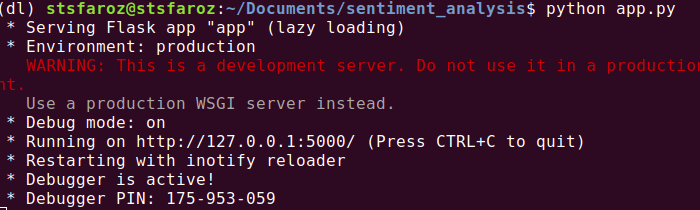
then open the jupyter or python editor and another side this server to be running parallel .

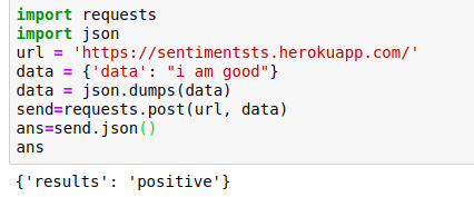
The main thing you have to keep in mind that we have to send the data in json format .

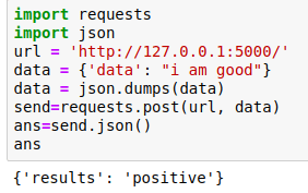
In this we just converted the data into json format

After that i just requested the running server with its address and passing the data with it.

We got answer as positive . It is working , Now we have to deploy this to Heroku.

Create a new account in Heroku if you did not have it

After Creating the account Click on new.

Click the Create new app

Then install the Heroku-CLI in your system

For windows 32bit https://cli-assets.heroku.com/heroku-x86.exe

Trending AI Articles:

1. How I used machine learning as inspiration for physical paintings

2. MS or Startup Job — Which way to go to build a career in Deep Learning?

3. TOP 100 medium articles related with Artificial Intelligence

4. Artificial Intelligence Conference

For windows 64bit https://cli-assets.heroku.com/heroku-x64.exe

For Ubuntu 16+ sudo snap install –classic heroku

For Mac brew tap heroku/brew && brew install heroku

For more info https://devcenter.heroku.com/articles/heroku-cli

Ok now we are ready to deploy but we need create two more files in it

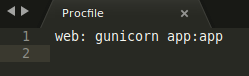
Procfile [P has to be in caps]

you can create the requirements.txt by this command

pip freeze > requirements.txt

We are ready to deploy it ,This is how our folder finally looks like

Then do the below steps in your cmd

$ heroku login

the it will popup the login in access in browser click login to it

$ cd sentiment_analysis/
$ git init
$ heroku git:remote -a sentimentsts

Deploy your application

Commit your code to the repository and deploy it to Heroku using Git.

$ git add .
$ git commit -am "make it better"
$ git push heroku master

Everything is done, Click the open app in your app page , you will get the link of the API

Finallyyyyy..

---

Deploying the machine learning model in Heroku using Flask was originally published in Becoming Human: Artificial Intelligence Magazine on Medium, where people are continuing the conversation by highlighting and responding to this story.

Via https://becominghuman.ai/deploying-the-machine-learning-model-in-heroku-using-flask-549c9ad0a47a?source=rss—-5e5bef33608a—4

Via https://becominghuman.ai/discover-the-best-of-ai-by-just-watching-videos-dd917031f3c4?source=rss—-5e5bef33608a—4

This freely available text on deep learning is fully interactive and incredibly thorough. Check out “Dive Into Deep Learning” now and increase your neural networks theoretical understanding and practical implementation skills.

Originally from KDnuggets https://ift.tt/2XMMLIm

In this article, we’ll walk through the detailed and helpful continuous integration (CI) that supports us in keeping StellarGraph’s demos current and informative.

Originally from KDnuggets https://ift.tt/2RIWADA

Also Exploratory Data Analysis for Natural Language Processing: A Complete Guide to Python Tools; A professor with 20 year experience to all high school seniors (and their parents). If you were planning to enroll in college next fall – don’t.

Originally from KDnuggets https://ift.tt/3eppHp0

From Human Vision to Computer Vision- Towards Spiked-Based Visual Intelligence and Neuromorphic Computing (4/4)

In the last story, I have talked about one of the most important breakthroughs in computer vision, the Convolutional Neural Networks (CNN). Today, CNNs are widely implemented into systems that require the processing of visual and spatial information and can be viewed as image features extractors and universal non-linear function approximators. They have achieved satisfying accuracy on complex tasks such as object recognition, semantic segmentation, depth and motion estimation, and visual odometry, which are crucial for the development of many visually-automated systems. However, human vision, by no means, is still unrivaled in terms of performance and robustness compared to that of the artificial vision, thus, prototypes of many systems today, e.g. automated driving system, still rely heavily on a diverse range of sensory systems to make up for this very limitation.

Moreover, as we progress and attempt to solve more advanced problems, increasing demand for computing and power resources became one of the most prominent issues for the CNNs as they require the extensive use of energy-intensive high-end graphic cards. The issue led to a shift in attention towards spiking neural networks (SNNs), a novel ANN inspired by the realistic neural dynamic of the brain. Aside from being known for their biologically plausible characteristics, they were also proven to be less computationally expensive than the conventional DNN and also show higher compatibility with dynamic event-based data, which could be apply to a real-time visual system. They are considered to be the third-generation neural network due to their event-driven, fast inference, and power-efficient nature.

So in this article, I wish to introduce you guys to novel Spiking Neural Networks (SNNs) and discuss how they, in combination with neuromorphic computing, could lead to a new breakthrough in achieving more dynamic and intelligent behavior in machine vision. It will also be the final article of the series, so I hope you guys enjoy it!

Visual Attention (VA) and Intelligence

One key element that differentiates the human’s vision from the current artificial vision is the ability to swiftly shift our focus and attention. In humans, divided attention allows the person to perform two or more tasks simultaneously and attentional shifting allows the person to quickly changes his focus and gain quick access to new information, thus, is expected that a high degree of divided attention and attentional shifting is associated with a high degree of intelligence. VA has long been extensively studied in computer vision and has been recognised as one of the crucial keys toward the next breakthrough in artificial intelligence.

So what makes visual attention so special and worth paying attention to? In both natural or artificial vision systems, raw sensory inputs are captured for further processing. Due to the immense amount of raw input available, the restriction of dataflow is crucial as it could overload the real-time computational possibility of the processing system. In humans, different mechanisms of data reduction are used, such as a motor shift of eyes or camera toward a certain object or entity (stimuli) localised in the visual field, which is known as overt attention. On the other hand, covert attention relies on the selection of information without any eye movements, only shifting the attention mentally. This selectivity allows the visual system to pay attention only to object(s) that are considered to be important at that specific moment in time while ignoring the rest of the less significant stimuli. This reduces the computational power immensely as the system no longer has to process through every single stimulus presented in the visual field. Therefore, it can be said that the core objective of visual attention is to achieve the least possible amount of visual information to be processed to solve complex high-level tasks, e.g., object recognition.

The General problems of VA in machine vision:

1. How can the system know what information is significant enough?
2. How does the visual system know when and how to direct attention and select significant information rather than doing so randomly?
3. Where is (are) the next potential target(s) of visual attention shifts? That is, how does it know where to actually focus its attention to?

Before anyone attempts to answer the questions above, it is important to first understand the pipeline of the natural visual system how such mechanism could be used to develope selective attention model in artificial vision.

Towards Event-Based Vision

Computer vision tasks primarily involve primarily of processing static images (or sequences of them such as frames in a video), the biological vision has shown to processes and emits fewer signals, mainly of changes occurring in the environment at a certain point in time. In simple words, cells in your eye only convey information to the brain when they detect a change in the scene — an event, while report nothing at all when no changes are detect. This key characteristic of biological vision systems allows the selective focus of attention on the salient portions of the scene, drastically reducing the amount of information that needs to be processed. Take an example of the frames captured from a video below.

In conventional sensors, data is conveyed in frames, which includes everything presented on the image is processed including sky, trees, and grass, while the only important information is actually the movement of the person, the swing of the golf club, and the movement of the ball. To avoid this issue of overprocessing irrelevant information, event-based sensors were introduced. Event-based sensors send out data packages, or events, from each pixel asynchronously whenever a local brightness change is detected in the pixel, rather than reading every single pixel and sending out frames at a constant rate. Such event-based sensing allows us to perform some vision tasks extremely efficiently, reducing the amount of required computation, transmitted data, and power consumption. Researchers have also shown that collecting statistics on event-based sensors could pave the way to full visual reconstruction. This is also where spiking neural networks steps in.

Spiking Neural Network and Neuromorphic Computing

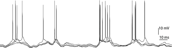
In accordance with what was mentioned in the last article, the picture above depicts a biological neuron and how they communicate with one another via action potential (which produces what known as ‘spikes’). A collection of spikes through time is known as spike train, as shown in the image below. They can be thought of as a collection of data (which in this case, is a function of time)

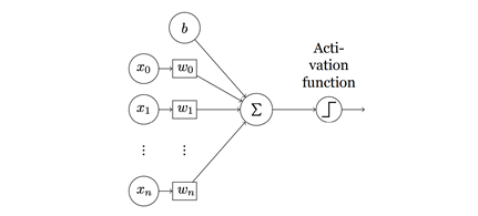
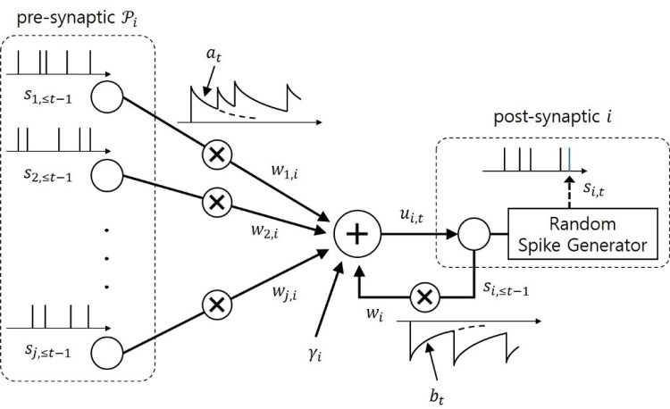
In traditional ANNs, the non-spiking neurons (see Fig 1.1) use differentiable, non-linear activation functions to propagate information between units, which allow units to be stacked into multiple layers.

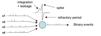
The derivative property of these neurons is also what makes learning through backpropagation via gradient-based optimization possible. The main difference between the traditional ANNs and the SNNs is that the SNNs adopt “spiking neurons”, which uses pulses of “spike” as the mean of communication, propagating information between units over time in a brain-like manner instead of using continuous activation value (see Fig 1.2 and 1.3). This spatio-temporal property (def: involving space and time) of the spiking neurons is also what makes SNN one of the most promising candidates to process temporal-dynamic visual data captured as a function of time by event-based sensors as well as in classical frame-based machine vision applications such as object recognition or detection, where they have proven to be accurate, fast, and efficient, especially when being run on neuromorphic hardware

The network was initially developed in order to shed some light on the computing dynamic of the brain. Interestingly, in terms of engineering motivation, SNNs also hold apparent advantages over traditional neural networks regarding performance speed and power-consumption when implemented on neuromorphic hardware platforms, which could resolve the power-consumption issue faced by CNN. This is due to the unique nature of the networks in which output spike trains can be made sparse in time. Since each spike would consume energy, having few spikes which contains high information content could effectively lower the total 6energy consumption. Neuromorphic systems and hardware design are also based on this spiking property and together with the implementation of SNNs, neuromorphic systems could play the key role in the progression of next-generation artificial intelligence.

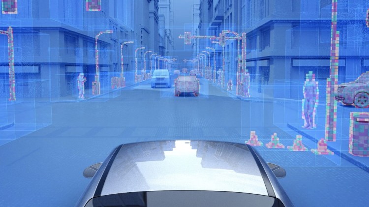
Since SNNs is proven effective at processing sensor information in real-time, it could become extremely beneficial in a dynamical visual system such as autonomous vehicles where it could improve the emergency brake assistants in which challenging weather condition as well as suddenly appearing vehicle or pedestrian are the main risk factors during high-speed maneuvering.

Aside from selective attention model, In recent years, various models of SNNs have been proposed to solve object recognition tasks, including the hybrid type such as the Convolution Spiking Neural Network that adopts conversion algorithms on the conventional CNN, in which weights are converted into spike signal input with leaks and refractory period. The main idea behind this hybrid architecture is to replace the CNN classifier unit with a spiking neuron whose firing rate is correlated with the output of that unit (shown in image above).

Trending AI Articles:

1. Cheat Sheets for AI, Neural Networks, Machine Learning, Deep Learning & Big Data

2. Data Science Simplified Part 1: Principles and Process

3. Getting Started with Building Realtime API Infrastructure

4. Artificial Intelligence Conference

The Current Limitation

Despite the promising potential, in practice, SNNs has a very challenging drawback where learning was proven difficult to train, especially when the network becomes multi-layer. One of the reasons being the lack of effective training and learning algorithms as the spike function adopted by the neurons is non-differentiable while backpropagation mechanism, which uses the derivative property of the neurons to train ANNs in a supervised manner, is what made the CNN one of the most, if not, the most powerful object classification/recognition tool to date. Many researchers believed that the performance of SNNs can be improved to catch up with that of ANNs by embedding the deep architecture into the network (Machado, Cosma, and McGinnity, 2019; Tavanaei et al, 2019; Xu, 2019). In order to mend this gap between ANN continuous-valued networks SNN, there is a crucial need to develop learning methods that could support deep (multi-layer) SNN with low error rates as their conventional counterparts. Successful approaches have been shown which include direct training of SNNs using backpropagation and applying stochastic gradient descent on to the SNN classifier layers (Stromatias et al., 2017). Spike-Timing Dependent Plasticity (STDP), a learning rule inspired by the plasticity algorithm of the brain that could be applied in both supervised and unsupervised manner, are also extensively studied due to its biologically plausible nature and possible implementation of low-power on-chip local learning.

Conclusion and Remarks

As one can see, we are now one step closer to achieving the biological-like vision. We have come a long way from a simple neural network to CNN, and eventually, to SNN. While CNN is perfect for object recognition in static images, it lacks a dynamic nature to process real-time datasets from newly developed event-based sensors which are dependant on time, thus making SNN a more promising candidate for real-time object recognition and processing task. Moreover, many studies have shown that SNNs have a potential to replace the power-hungry CNN as the spiking algorithms can be implemented on neuromorphic systems.

I hope everyone who read through the series now has a better idea of the progression in computer vision and how neuroscience had greatly contributed to the breakthrough of such a fascinating field (and will continue to do so). In the next article, I will dive deeper into the technical property of Spiking Neural Network including the encoding and learning rules. I have left a list of references that I used in this article which could be served as additional readings for those who are interested. Do share my article if you find it useful. See you next time!

Don’t forget to give us your ? !

---

From Human Vision to Computer Vision- Towards Spiked-Based Visual Intelligence and Neuromorphic… was originally published in Becoming Human: Artificial Intelligence Magazine on Medium, where people are continuing the conversation by highlighting and responding to this story.

Via https://becominghuman.ai/from-human-vision-to-computer-vision-towards-spiked-based-visual-intelligence-and-neuromorphic-913e5de21bf9?source=rss—-5e5bef33608a—4