
In the mid-90s, a variation of recurrent net with so-called Long Short-Term Memory units, or LSTMs, was proposed by the German researchers Sepp Hochreiter and Juergen Schmidhuber as a solution to the vanishing gradient problem.
LSTMs help preserve the error that can be backpropagated through time and layers. By maintaining a more constant error, they allow recurrent nets to continue to learn over many time steps (over 1000), thereby opening a channel to link causes and effects remotely. This is one of the central challenges to machine learning and AI, since algorithms are frequently confronted by environments where reward signals are sparse and delayed, such as life itself. (Religious thinkers have tackled this same problem with ideas of karma or divine reward, theorizing invisible and distant consequences to our actions.)
LSTMs contain information outside the normal flow of the recurrent network in a gated cell. Information can be stored in, written to, or read from a cell, much like data in a computer’s memory. The cell makes decisions about what to store, and when to allow reads, writes and erasures, via gates that open and close. Unlike the digital storage on computers, however, these gates are analog, implemented with element-wise multiplication by sigmoids, which are all in the range of 0–1. Analog has the advantage over digital of being differentiable, and therefore suitable for backpropagation.
Those gates act on the signals they receive, and similar to the neural network’s nodes, they block or pass on information based on its strength and import, which they filter with their own sets of weights. Those weights, like the weights that modulate input and hidden states, are adjusted via the recurrent networks learning process. That is, the cells learn when to allow data to enter, leave or be deleted through the iterative process of making guesses, backpropagating error, and adjusting weights via gradient descent.

Successful LSTM models have been built on a huge number of datasets. These include the models powering large-scale speech and translation services (Hochreiter & Schmidhuber, 1997)


The reason why there is a need for LSTM s is that RNNs have difficulties in terms of remembering context across longer sequences.
LSTMs are very well suited to avoid the long-term dependency problem. Their default behavior is to keep information for long periods of time, so there is no struggle for them to learn.
Contextual information which can be accessed by standard RNNs restricted due to the fact that the influence of a given input on the hidden layer, and therefore on the network output, either decays or blows up exponentially as it cycles around the network’s recurrent connections. As mentioned above this is referred to as the vanishing gradient problem. LSTM is specifically designed to address the vanishing gradient problem. The following statements by Gers et al., 2000 are worth to emphasize when it comes understanding LSTMs:
“Standard RNNs fail to learn in the presence of time lags greater than 5–10 discrete time steps between relevant input events and target signals. LSTM can learn to bridge minimal time lags in excess of 1000 discrete time steps by enforcing constant error ow through “constant error carrousels” (CECs) within special units, called cells.”
Top 4 Most Popular Ai Articles:
2. Explained in 5 MinutesHow To Choose Between Angular And React For Your Next Project
LSTM architecture was motivated by an analysis of error flow in existing RNNs which discovered that long time lags were inaccessible to existing architectures, because backpropagated error either blows up or decays exponentially.
An LSTM layer consists of a set of recurrently connected blocks, known as memory blocks. These blocks can be thought of as a differentiable version of the memory chips in a digital computer. Each one contains one or more recurrently connected memory cells and three multiplicative units — the input, output and forget gates — that provide continuous analogues of write, read and reset operations for the cells.
Learning rate and network size are the most crucial tunable LSTM hyperparameters which can be tuned independently. The learning rate can specifically be calibrated first using a fairly small network, thus saving a lot of experimentation time.
Let’s see how LSTMs function in detail now. You would remember from the previous chapters that that RNNs possess a chain of repeating modules of neural network, usually in the form of a single tanh layer.
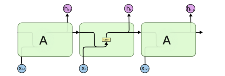
The repeating module in LSTMs is a bit different as instead of having a single neural network layer, there are four of them, all of which are interacting in a very special way.

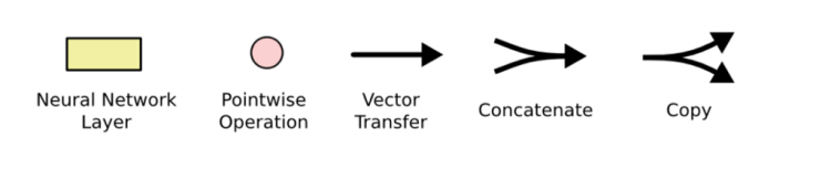
In the figure above, the pink circles represent pointwise operations, like vector addition, while the yellow boxes are learned neural network layers. Lines merging denote concatenation, while a line forking denote its content being copied and the copies going to different locations. Starting from the output of one node to the inputs of others, each line carries an entire vector from the output of one node to the inputs of others.
So, LSTMs keep adding memory gates that control when memory is saved from one iteration to the next. The activation of these gates is controlled by means of connection weights. Special units called memory blocks in the recurrent hidden layer entail (Koenker et al, 2001):
○ Memory cells
○ Multiplicative units called gates
■ Input gate: controls flow of input activations into memory cell
■ Output gate: controls output flow of cell activations
■ Forget gate: process continuous input streams
Let’s look at each steps on how the LSTM works (Koenker et al, 2001):
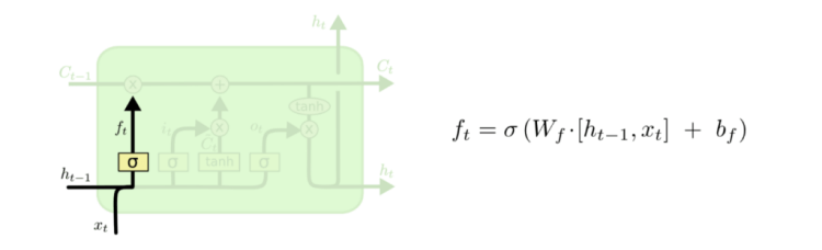
– A decision should be made what information needs to be thrown away from the cell state. A sigmoid layer called the “forget gate layer” looks at ht−1 and xt and outputs a number between 0 and 1 for each number in the cell state Ct−1. While ‘1’ denotes “completely keep this” ‘0’ represents “get rid of this completely.”
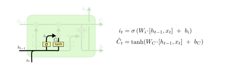
– The next step is to decide what new information should be stored in the cell state.
– First, a sigmoid layer called the “input gate layer” decides which values are to be updated.
– Next, a tanh layer creates a vector of new candidate values, C̃t, that could be added to the state.
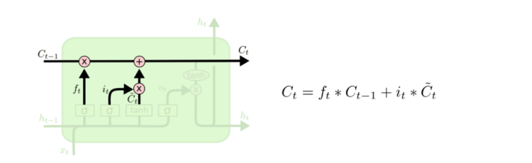
– The old cell state, Ct−1, should be updated into the new cell state Ct. The previous steps already decided what to do, so one only needs to multiply the old state by ft, forgetting the things decided to be forgotten earlier. Then, one should add it∗C̃t. This is the new candidate values, scaled by how much it is decided to update each state value.
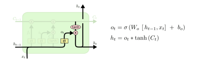
– Finally, a decision should be made regarding the output. This output will be based on a filtered version of the cell state.
– First, one would need a sigmoid layer which decides what parts of the cell state to output.
– Then, one would need to put the cell state through Tanh (to push the values to be between −1 and 1) and multiply it by the output of the sigmoid gate to get the related outputs
Variants on Long Short Term Memory
The last section provided an overview of a generic LSTM, yet not all LSTMs might be the same. One of the most popular variation of LSTM is the so called “peephole connection”. It refers to letting the gate layers look at the cell state (Koenker et al, 2001).
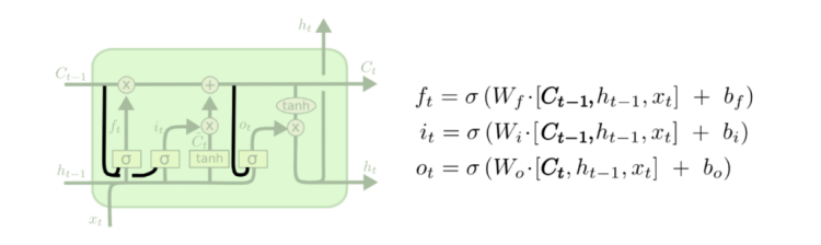
As it can be seen in the figure above, peepholes can be added to all the gates, although that is not necessarily the case.
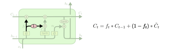
Another variant would be to use a combination of both coupled forget and input gates. Rather than separately determining what to forget and what to add, these decisions are made together. Forgetting occurs when a new input would be added into its place while new values will be added when something needs to be forgotten (Koenker et al, 2001).
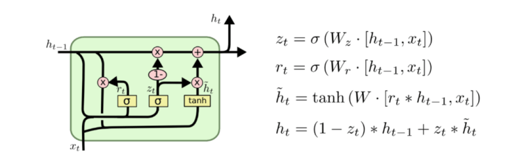
Another variation is the so called GRU (Gated Recurrent Unit) which combines both the forget and input gates into a single “update gate” by merging the cell and hidden states (Koenker et al, 2001). This model has been growing increasingly popular.
These examples are only a few variants for LSTM. There are many other variants. Yet, one question that you might want to ask is which variant would be the best to choose or whether these differences would matter at all. Once you have a response to this, you can realize that you already become an expert in neural networks.
Don’t forget to give us your ? !


The Logic of Digital Memories was originally published in Becoming Human: Artificial Intelligence Magazine on Medium, where people are continuing the conversation by highlighting and responding to this story.
Via https://becominghuman.ai/the-logic-of-digital-memories-b6ec8feb7555?source=rss—-5e5bef33608a—4
source https://365datascience.weebly.com/the-best-data-science-blog-2020/the-logic-of-digital-memories