Beyond hypethe reality of a Machine Learning project

Beyond hype — the reality of a Machine Learning project

Machine Learning (ML) is one of the fundamental components of data science. Many data problems can be framed as ML problems.

If you have studied ML, you are familiar with some of its most famous success stories, such as churn prediction, fault detection, fraud detection, search engines and recommendation systems; you may not yet be aware of everything that goes behind making an ML project successful.

In this article I will lift the veil on some of the crucial ingredients of making machine learning as effective as it can be.

Big Data Jobs

A process model for ML projects

Learning the technology typically starts with the basic building blocks: how to convert a business problem into data that can be processed by an ML algorithm; how to train the algorithm (with tools such as automl); how to fill the role of an Analytics Translator (AT), whose main focus is — tech to business operationalization. Those steps, while essential, are only part of a much larger ML lifecycle model. The model is pictured below, and every ML user should be aware of it.

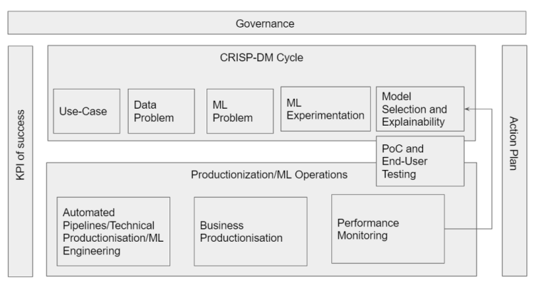
All steps of the process must be managed by a centralized governance department, directly under a Chief Analytics Officer or Chief Data Officer. The governance team typically consists of product owners and managers, data security experts, privacy experts, compliance experts and regulatory members.

Key steps in making an ML project succeed

Here are the team roles and essential details of each step appearing in the figure.

Use case: This is one of the most critical steps in the entire ML lifecycle. Its purpose is to ask fundamental questions before you dive into the technical tasks of data and ML (and to decide whether to do so!). Such questions include:

  • What is the problem we are trying to solve?
  • Is it really a ML problem, or will analytics or classical statistics be more effective?
  • If we get the model, how will it be used?
  • What are our KPIs of success? (Better define them ahead of time than worry about the success indicators after the application has been written, they can be updated during the experimentation phase).
  • Who are the end-users and how will they interact with the application?

Trending AI Articles:

1. Why Corporate AI projects fail?

2. How AI Will Power the Next Wave of Healthcare Innovation?

3. Machine Learning by Using Regression Model

4. Top Data Science Platforms in 2021 Other than Kaggle

Roles required at this step: analytics translator, data scientist (can serve as translator), product owner, governance team.

Data problem: This step maps business onto data by asking the following questions:

  • What are the inputs and outputs? Where is the data stored?
  • How much data do we need? Do we have enough labelled data? Do we need to collect data?
  • What can we assume about the quality of the data?
  • How will data be fed into such a system (batch vs stream, online vs offline, on demand vs forecast, static vs dynamic)?

ML problem: If the steps above are well defined, this part is rather easy to work out. Most ML problems fall into one of two categories: supervised (regression or classification) and unsupervised learning. For an ML practitioner, it helps to know about new ML approaches such as semi-supervised learning and active learning. An ML practitioner needs to know how ML algorithms work. Specific questions to ask are:

  • What kind of ML problem do we have?
  • How do we define KPIs of success at every step in the process (including: data quality, ML metrics, business metrics, prediction scores, error margins)?
  • Is explainable ML needed?
  • How will the output flow to the end-user?
  • Do we care about the kind of algorithm we use?
  • What tools will we use?

While most ML practitioners are data scientists, most ML problems only require knowledge of applied machine learning. The general set of skills needed at this step include coding ability, experience with statistics, understanding of different ML models, knowledge of experimentation frameworks such as mlops, experience with cloud computing, and experience with automl.

Roles required at this step: Applied Machine Learning practitioner, data scientist, Web/mobile app developer, and preferably a statistician.

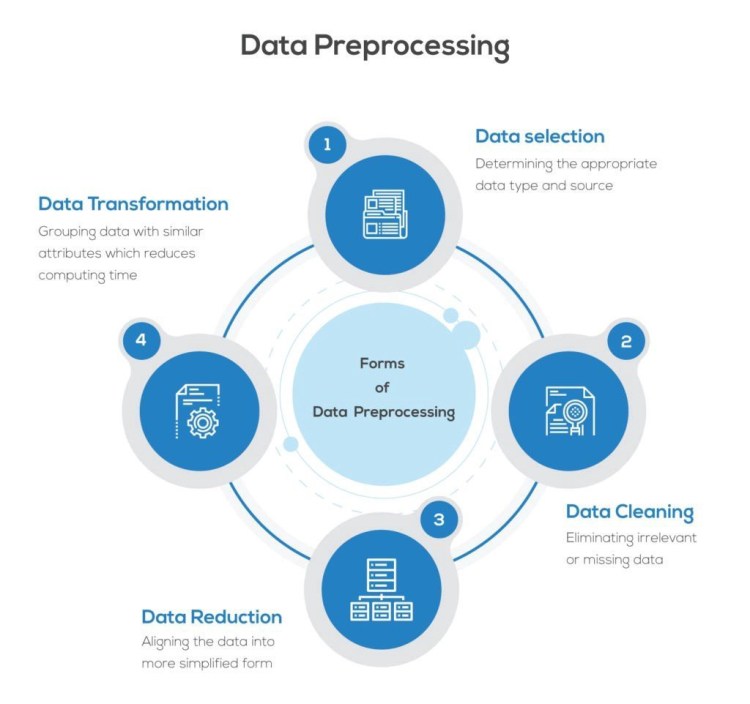
ML experimentation: This is a classical experimentation step involving data exploration, cleaning, feature engineering, model development and experiment tracking (AutoML platforms lik modulos [2] help here). A 80–20 rule applies here: 80% cleaning plus feature engineering, 20% model building.

Model Selection, Explainability and Bias: Most parts of model development and selection can be automated using standard Python libraries (including again automl). Open-source libraries are already available to help explainability and bias analysis, and new ones are appearing all the time. Cloud providers are trying to take the lead in the race to automate the full process.

Proof of ConceptContext and End-User Testing: Before going into production, you will often create a Proof of Concept, which can consist of testing the integration of model output into the system, or just of building a simple web application around the model so that end-users can run the results and provide feedback. In a fully functional and productionized user app, one needs to bring in UX/UI designers as well. For this step you will need to have A/B and A/A testing skills available.

“Pioneer” AI organizations [1] with well-established data processes have put in place frameworks and documented instructions for most of the above steps. Though cloud service providers try to provide standardized pipelines to attract companies at this stage, most organizations are using some form of hybrid-cloud model and need access to 3rd party platforms like omega|ml [3].

ML Operations: A machine-learning project is not just a technical IT endeavor. Particularly when it reaches the deployment and operation step, it also involves business aspects. The complexity of ML operations depends upon such factors as: how often should the ML model be trained? How will the ML model be used in the end-product? How many end-users will the product handle?

Roles required at this step: data engineers, data scientists, business analysts, analytics translators, ML engineers, data product owners, end users.

Model engineering: This step requires good engineering knowledge and exposure to technological stacks that include CI/CD pipelines, DataOps, MLOps, Data Engineering and data Containerization engines.. In this vibrant area, where new ways to automate the process continue to appear regularly, you will again require a mix of engineering and business skills. The most successful AI organizations organize all projects around a well-defined ML engineering pipeline.

Business productization: This step is devoted to making sure the machine-learning solution is closely integrated with the business aspects. As a result, it too requires a mix of business and engineering skills and some user testing. It should involve people with expertise from both sides of the aisle, in particular the business professionals who will be using the output of ML algorithms.

Performance monitoring: The purpose of this step, which is also called post-production monitoring, is to assess how the ML solution actually works. It involves tracking the evolution of a number of parameters over time: modeling and business KPIs as well as data-related aspects, particularly data, concept and covariate drift. Without this step, there is a risk that an initially adequate ML system will progressively degrade because the training set no longer reflects the current data. Effective performance monitoring enables the data owner to trigger appropriate recalibration processes if this phenomenon passes a certain statistical threshold.

Governance: Any ML-based system must include, during development and after deployment, a strong governance system defining KPIs and action plans in response to possible hiccups. Governance should be under the domain of a governing body directly under the Chief Data Officer or Chief Analytics Officer.

Towards a holistic view of the ML process and its integration into the business process

In spite of all the hype around AI, many companies are still struggling to profit from AI. Why is that and what can you do about it? A core reason is the dire shortage of people who understand the full process as outlined above — taught, in full depth, in Propulsion’s courses.

We developed Propulsion’s ML course [4] by leveraging the experience of over 60 ML projects delivered over the past four years across a wide range of Swiss companies and industries. The course also relies on extensive market research to identify areas leading to ML failures in organizations.
The result is a course that integrates not only the latest and brightest ML tools and techniques, at the forefront of today’s rapidly evolving ML technology, but also numerous elements that you cannot get by studying technology alone: all the business aspects, rooted in an in-depth understanding of what makes ML succeed or fail in a company.

This is the kind of hot skill that companies badly need today. If you are interested in acquiring it to make your future employer’s ML projects be part of the success stories, we look forward to receiving your applications. If you like this article (and the others on this blog), please share it in your network!

[1]. Propulsion Academy Blog: Whom should organizations re-skill or hire to succeed in the age of AI and how to become an AI Pioneer?
[2]. modulos
[3]. omega|ml
[4]. Propulsion Academy Machine Learning course

Don’t forget to give us your ? !


Beyond hype — the reality of a Machine Learning project was originally published in Becoming Human: Artificial Intelligence Magazine on Medium, where people are continuing the conversation by highlighting and responding to this story.

Via https://becominghuman.ai/beyond-hype-the-reality-of-a-machine-learning-project-ea79b57e0c46?source=rss—-5e5bef33608a—4

source https://365datascience.weebly.com/the-best-data-science-blog-2020/beyond-hypethe-reality-of-a-machine-learning-project

How To Prepare Data For OCR Learning

Data analysis without data preparation is a myth. Unless we feed the right data in a proper format, Machine Learning algorithms won’t be able to solve our problem. If we give one wrong input then we end up where we started. So it’s very important to understand what data preparation is and how one can do it.

Data, in its original form, may have a lot of missing pieces or disarrangement. Through data processing, one can modify this raw information from a specific database to a format that is understandable and which the machine can learn. Mentioned below are the ways that, we at Infrrd , employ in preparing our data.

1. Data Selection:

It is necessary first to identify the type of data we are going to be working with. One has to keep in mind whether the available data will be able to address an existing problem or not. We keep certain factors in consideration before selecting the data:

  • Data should not be of low quality: Low-quality input= low-quality output.
  • Dataset is not error-ridden: The more the errors the more time it consumes to preprocess it.
  • Dataset is unbiased: Having an unbiased dataset opens new doors in terms of discoveries in predictive modeling.
Big Data Jobs

2. Data Preprocess:

Once we have selected the data, we determine how we will be using it. In this step, we transform the data into a format that would be compatible with our future use. There are 3 ways to preprocess data:

  • Format: Since the raw input is not in a usable format for OCR learning, formatting it ensures that machine learning algorithms can comprehend it to solve the issue. For example, the formats of date and time, etc. need to be consistent throughout the dataset.
  • Cleanse: Here we remove the missing data or the irrelevant ones. It also involves fixing structural errors like typos and inconsistent capitalization, mislabeled classes, etc. Here data wrangling tools, or batch processing through scripting becomes essential.
  • Sampling: Often there is more information available to us than we actually require. Via sampling, we obtain a smaller portion of the data which gives us prompt prototype results from the algorithms and speeds up the entire data mining process for OCR learning.

Trending AI Articles:

1. Why Corporate AI projects fail?

2. How AI Will Power the Next Wave of Healthcare Innovation?

3. Machine Learning by Using Regression Model

4. Top Data Science Platforms in 2021 Other than Kaggle

3. Data Transformation:

This is the final step wherein we receive the modified data for machine learning. Sometimes we may need to go back to preprocessing information just to make sure that we have the right kind of information for the specific algorithm or problem domain we are working on. There are 3 data transformation procedures that we use:

  • Centre & Scale: Preprocessed data will more likely contain a mix of scales such as currencies, weight, height, etc. By centering and scaling the data using mean and standard deviation respectively, these variables could be standardized.
  • Decompose: Through this procedure, complex data concepts are fragmented and segregated into more specific segments to achieve a more useful machine learning format. It is also called data bucketing.
  • Aggregate: This step allows information to be gathered and expressed in a summarized pattern. The bulk data can be grouped by segmenting it into broader aggregates with similar attributes reducing data size and computing time.
  • In general, data preparation is a big, non-fancy task in OCR machine learning, involving some repetition, exploration, and inspection. Using machine learning and NLP, we have built context around the prepared data for easy inference, to accurately extract and predict data simultaneously while learning from scores of datasets. Thus, the data extracted by Infrrd OCR is 50 times more accurate than any other OCR solution in the market.

Infrrd’s OCR has learned from scores of enterprise data, thereby, making its results more than 98% accurate for most samples. This can apply to many enterprise processes like:

  • Banking- Processing handwritten checks and documents
  • Finance- Invoice, receipts, and mortgage documents processing
  • Manufacturing- RFP processing
  • Healthcare- Insurance forms and general health forms processing

SCHEDULE A DEMO FOR INTELLIGENT DATA EXTRACTION

Don’t forget to give us your ? !


How To Prepare Data For OCR Learning was originally published in Becoming Human: Artificial Intelligence Magazine on Medium, where people are continuing the conversation by highlighting and responding to this story.

Via https://becominghuman.ai/how-to-prepare-data-for-ocr-learning-ba131b83857b?source=rss—-5e5bef33608a—4

source https://365datascience.weebly.com/the-best-data-science-blog-2020/how-to-prepare-data-for-ocr-learning

Pneumonia Detection using CNN

Detecting whether someone suffers pneumonia based on their chest x-ray images.

Several x-ray images in the dataset used in this project.

Hey there! Just finished another deep learning project several hours ago, now I wanna share what I actually did there. So the objective of this challenge is to determine whether a person suffers pneumonia or not, and if yes, then determine whether it’s caused by bacteria or virus. — Well, I think this project should be called as classification instead of detection. — In other words, this task is going to be a multiclass classification problem where the label names are: normal, virus and bacteria. In order to solve this problem, I decided to use CNN (Convolutional Neural Network) thanks to its excellent ability to perform image classification. Not only that, here I also implement image augmentation technique as an approach to improve model performance. By the way, here I obtained 80% of accuracy on test data which is pretty impressive to me.

The dataset used in this project can be downloaded from this Kaggle link. The size of the entire dataset itself is around 1 GB, so it might take a while to download. Or, we can also directly create a Kaggle Notebook and code the entire project there, so we don’t even need to download anything. Next, if you explore the dataset folder, you will see that there are 3 sub folders, namely train, test and val. Well, I think those folder names are self-explanatory. In addition, the data in train folder consists of 1341, 1345 and 2530 samples for normal, virus and bacteria class respectively. I think that’s all for the intro, let’s now jump into the code!

Note: I put the entire code used in this project at the end of this article.

Big Data Jobs

Loading modules and train images

The very first thing to do when working with computer vision project is to load all required modules and the image data itself. I use tqdm module to display progress bar which you’ll see why it is useful later on. The last import I do here is ImageDataGenerator coming from Keras module. This module is going to help us implementing image augmentation technique during the training process.

import os
import cv2
import pickle
import numpy as np
import matplotlib.pyplot as plt
import seaborn as sns
from tqdm import tqdm
from sklearn.preprocessing import OneHotEncoder
from sklearn.metrics import confusion_matrix
from keras.models import Model, load_model
from keras.layers import Dense, Input, Conv2D, MaxPool2D, Flatten
from keras.preprocessing.image import ImageDataGenerator
np.random.seed(22)

Next, I define two functions to load image data from each folder. The two functions below might look identical at glance, but there’s actually a little difference at the line with bold text. This is done because the filename structure in NORMAL and PNEUMONIA folders are slightly different. Despite the difference, the other process done by both functions are essentially the same. First, all images are going to be resized to 200 by 200 pixels large. This is important to do since the images in all folders are having different dimensions while neural network can only accept data with fixed array size. Next, basically all images are stored with 3 color channels, which is I think it’s just redundant for x-ray images. So the idea here is to convert all those color images to grayscale.

# Do not forget to include the last slash
def load_normal(norm_path):
norm_files = np.array(os.listdir(norm_path))
norm_labels = np.array(['normal']*len(norm_files))

norm_images = []
for image in tqdm(norm_files):
image = cv2.imread(norm_path + image)
image = cv2.resize(image, dsize=(200,200))
image = cv2.cvtColor(image, cv2.COLOR_BGR2GRAY)
norm_images.append(image)

norm_images = np.array(norm_images)

return norm_images, norm_labels

def load_pneumonia(pneu_path):
pneu_files = np.array(os.listdir(pneu_path))
pneu_labels = np.array([pneu_file.split('_')[1] for pneu_file in pneu_files])

pneu_images = []
for image in tqdm(pneu_files):
image = cv2.imread(pneu_path + image)
image = cv2.resize(image, dsize=(200,200))
image = cv2.cvtColor(image, cv2.COLOR_BGR2GRAY)
pneu_images.append(image)

pneu_images = np.array(pneu_images)

return pneu_images, pneu_labels

As the two functions above have been declared, now we can just use it to load train data. If you run the code below you’ll also see why I choose to implement tqdm module in this project.

norm_images, norm_labels = load_normal('/kaggle/input/chest-xray-pneumonia/chest_xray/train/NORMAL/')
pneu_images, pneu_labels = load_pneumonia('/kaggle/input/chest-xray-pneumonia/chest_xray/train/PNEUMONIA/')
Progress bar displayed using tqdm module.

Up to this point, we already got several arrays: norm_images, norm_labels, pneu_images and pneu_labels. The one with _images suffix indicates that it contains the preprocessed images while the array with _labels suffix shows that it stores all ground truths (a.k.a. labels). In other words, both norm_images and pneu_images are going to be our X data while the rest are going to be y data. To make things look more straightforward, I decided to concatenate the values of those arrays and store in X_train and y_train array.

X_train = np.append(norm_images, pneu_images, axis=0)
y_train = np.append(norm_labels, pneu_labels)
The shape of the features (X) and labels (y).

By the way I obtain the number of images of each class using the following code:

Finding out the number of unique values in our training set.

Displaying several images

Well, displaying several images like what I wanna do in this stage is not mandatory. But I just wanna do this anyway just to ensure whether the pictures are already loaded and preprocessed well. The code below is used to display 14 images taken randomly from X_train array along with the labels.

fig, axes = plt.subplots(ncols=7, nrows=2, figsize=(16, 4))

indices = np.random.choice(len(X_train), 14)
counter = 0

for i in range(2):
for j in range(7):
axes[i,j].set_title(y_train[indices[counter]])
axes[i,j].imshow(X_train[indices[counter]], cmap='gray')
axes[i,j].get_xaxis().set_visible(False)
axes[i,j].get_yaxis().set_visible(False)
counter += 1
plt.show()
Some of the preprocessed x-ray images.

We can see the figure above that all images are now having the exact same size — unlike the one that I use for the cover picture of this post.

Loading test images

As we already know that all train data have been loaded successfully, we can now use the exact same function to load our test data. The steps are pretty much the same, but here I store those loaded data in X_test and y_test array. The data used for testing itself contains 624 samples.

norm_images_test, norm_labels_test = load_normal('/kaggle/input/chest-xray-pneumonia/chest_xray/test/NORMAL/')
pneu_images_test, pneu_labels_test = load_pneumonia('/kaggle/input/chest-xray-pneumonia/chest_xray/test/PNEUMONIA/')
X_test = np.append(norm_images_test, pneu_images_test, axis=0)
y_test = np.append(norm_labels_test, pneu_labels_test)

Furthermore, I notice that it takes pretty long just to load the entire dataset. Hence I decided to save X_train, X_test, y_train and y_test in separate file using pickle module, so that I don’t need to repeat running the codes above next time I wanna use these data again.

# Use this to save variables
with open('pneumonia_data.pickle', 'wb') as f:
pickle.dump((X_train, X_test, y_train, y_test), f)
# Use this to load variables
with open('pneumonia_data.pickle', 'rb') as f:
(X_train, X_test, y_train, y_test) = pickle.load(f)

Since all X data have been preprocessed well, now it’s time to work with labels y_train and y_test.

Label preprocessing

At this point, both y variables consist of either normal, bacteria or virus written in string datatype. In fact, such labels are just not acceptable by neural network. Therefore, we need to convert that into one-hot format. Luckily we got OneHotEncoder object taken from Scikit-Learn module which is extremely helpful to do the conversion. In order to do that, we need to begin with creating new axis on both y_train and y_test. (We create this new axis since that’s just the shape expected by OneHotEncoder).

y_train = y_train[:, np.newaxis]
y_test = y_test[:, np.newaxis]

Next, initialize one_hot_encoder like this. Notice that here I pass False as the sparse argument to make the next step kinda simpler. But if you wanna use sparse matrix instead, just go with sparse=True or leave the parameters empty.

one_hot_encoder = OneHotEncoder(sparse=False)

Finally we are going to use this one_hot_encoder to actually convert these y data into one-hot. The encoded labels are then stored in y_train_one_hot and y_test_one_hot. These two arrays are the labels that we will use for the training.

y_train_one_hot = one_hot_encoder.fit_transform(y_train)
y_test_one_hot = one_hot_encoder.transform(y_test)

Reshaping X data into (None, 200, 200, 1)

Now let’s get back to our X_train and X_test. It’s important to know that the shape of these two arrays are (5216, 200, 200) and (624, 200, 200) respectively. Well, at glance, these two shapes look fine as we can just display that using plt.imshow() function. However though, this shape is just not acceptable by convolution layer since it expects color channel to be included as its input. Thus, since this image is essentially colored in grayscale, then we need to add a new axis with 1 dimension which is going to be recognized by the convolution layer as the only color channel. The implementation is not as complicated as my explanation though:

X_train = X_train.reshape(X_train.shape[0], X_train.shape[1], X_train.shape[2], 1)
X_test = X_test.reshape(X_test.shape[0], X_test.shape[1], X_test.shape[2], 1)

Now after running the code above, if we check the shape of both X_train and X_test, then we will see that the shape is now (5216, 200, 200, 1) and (624, 200, 200, 1) respectively.

Trending AI Articles:

1. Why Corporate AI projects fail?

2. How AI Will Power the Next Wave of Healthcare Innovation?

3. Machine Learning by Using Regression Model

4. Top Data Science Platforms in 2021 Other than Kaggle

Data augmentation

Here’s the part where I have never been working with. So this is my very first time doing data augmentation for image classification task.

Anyway, the main point of augmenting data — or more specifically augmenting train data — is that we are going to increase the number of data used for training by creating more samples with some sort of randomness on each of them. Those randomness might include translations, rotations, scaling, shearing and flips. Such technique is able to help our neural network classifier to reduce overfitting, or in other words, it can make the model generalize data samples better. Luckily, the implementation is very easy thanks to the existence of ImageDataGenerator object which can be imported from Keras module.

datagen = ImageDataGenerator(
rotation_range = 10,
zoom_range = 0.1,
width_shift_range = 0.1,
height_shift_range = 0.1)

So what I essentially do in the code above is to set the range of randomness. Here’s a link to the documentation of ImageDataGenerator if you wanna know the details of each argument. Next, what we need to do after initializing the datagen object is to fit it with our X_train. This process is then followed by applying flow() method in which this step is useful such that train_gen object is now able to generate batches of augmented data.

datagen.fit(X_train)
train_gen = datagen.flow(X_train, y_train_one_hot, batch_size=32)

CNN (Convolutional Neural Network)

Now it’s time to actually build the neural network architecture. Let’s start with the input layer (input1). So this layer basically takes all the image samples in our X data. Hence we need to ensure that the first layer accepts the exact same shape as the image size. It’s worth noting that what we need to define is only (width, height, channels), instead of (samples, width, height, channels).

Afterwards, this input1 layer is connected to several convolution-pooling layer pairs before eventually being flattened and connected to dense layers. Notice that all hidden layers in the model are using ReLU activation function due to the fact that ReLU is faster to compute compared to sigmoid, and thus, the training time required is shorter. Lastly, the last layer to connect is output1, where it consists of 3 neurons with softmax activation function. Here softmax is used because we want the outputs to be the probability value of each class.

input1 = Input(shape=(X_train.shape[1], X_train.shape[2], 1))

cnn = Conv2D(16, (3, 3), activation='relu', strides=(1, 1),
padding='same')(input1)
cnn = Conv2D(32, (3, 3), activation='relu', strides=(1, 1),
padding='same')(cnn)
cnn = MaxPool2D((2, 2))(cnn)

cnn = Conv2D(16, (2, 2), activation='relu', strides=(1, 1),
padding='same')(cnn)
cnn = Conv2D(32, (2, 2), activation='relu', strides=(1, 1),
padding='same')(cnn)
cnn = MaxPool2D((2, 2))(cnn)

cnn = Flatten()(cnn)
cnn = Dense(100, activation='relu')(cnn)
cnn = Dense(50, activation='relu')(cnn)
output1 = Dense(3, activation='softmax')(cnn)

model = Model(inputs=input1, outputs=output1)

After constructing the neural network using the code above, we can display the summary of our model by applying summary() to model object. Below is how our CNN model looks like in details. We can see here that we got 8 million params in total — which is a lot. Well, that’s why I run this code on Kaggle notebook.

Summary of the CNN model.

Anyway, after the model being constructed, now we need to compile the neural net using categorical cross entropy loss function and Adam optimizer. So the loss function is used since it’s just the one that’s commonly used in multiclass classification task. Meanwhile, I choose Adam as the optimizer since it’s just the best one to minimize loss value in most neural network tasks.

model.compile(loss='categorical_crossentropy', 
optimizer='adam', metrics=['acc'])

Now it’s time to train the model! Here we are going to use fit_generator() instead of fit() because we are going to take the train data from train_gen object. — If you pay attention to the data augmentation part, you’ll notice that train_gen is created using both X_train and y_train_one_hot. Therefore, we don’t need to explicitly define the X-y pairs in the fit_generator() method.

history = model.fit_generator(train_gen, epochs=30, 
validation_data=(X_test, y_test_one_hot))

What’s so special with train_gen is that the training process is going to be done using samples with some randomness. So all training data that we have in X_train is not directly fed into the neural network. Instead, those samples are going to be used as the basis of the generator to generate new image with some random transformations. Moreover, this generator produces different images in each epoch which is extremely good for our neural network classifier to better generalize samples in test set. And well, below is how the training process goes.

Epoch 1/30
163/163 [==============================] - 19s 114ms/step - loss: 5.7014 - acc: 0.6133 - val_loss: 0.7971 - val_acc: 0.7228
.
.
.
Epoch 10/30
163/163 [==============================] - 18s 111ms/step - loss: 0.5575 - acc: 0.7650 - val_loss: 0.8788 - val_acc: 0.7308
.
.
.
Epoch 20/30
163/163 [==============================] - 17s 102ms/step - loss: 0.5267 - acc: 0.7784 - val_loss: 0.6668 - val_acc: 0.7917
.
.
.
Epoch 30/30
163/163 [==============================] - 17s 104ms/step - loss: 0.4915 - acc: 0.7922 - val_loss: 0.7079 - val_acc: 0.8045

The entire training itself took my Kaggle notebook around 10 minutes. So be patient! After being trained, we can plot the improvement of accuracy score and the decrease of loss value like this:

plt.figure(figsize=(8,6))
plt.title('Accuracy scores')
plt.plot(history.history['acc'])
plt.plot(history.history['val_acc'])
plt.legend(['acc', 'val_acc'])
plt.show()
plt.figure(figsize=(8,6))
plt.title('Loss value')
plt.plot(history.history['loss'])
plt.plot(history.history['val_loss'])
plt.legend(['loss', 'val_loss'])
plt.show()
Accuracy score improvement
Loss value decrease.

According to the two figures above, we can say that the performance of the model keeps improving, even though both the testing accuracy and loss value look fluctuating within this 30 epochs. Another important thing to notice here is that this model does not suffer from overfitting thanks to the data augmentation method we applied in the earlier part of this project. We can see here that the accuracy on train and test data are 79% and 80% respectively at the final iteration.

Fun fact: before implementing data augmentation method, I got 100% accuracy on train data and 64% on test data, which is extremely overfitting. So we can clearly see here that augmenting train data is very effective to both improve test accuracy score while at the same time also reduces overfitting.

Model evaluation

Now let’s deep dive into the accuracy towards test data using confusion matrix. First, we need to predict all the X_test and convert the result back from one-hot format to its actual categorical label.

predictions = model.predict(X_test)
predictions = one_hot_encoder.inverse_transform(predictions)

Next, we can employ confusion_matrix() function like this:

cm = confusion_matrix(y_test, predictions)

It’s important to pay attention that the arguments used in the function is (actual, predicted) — not the other way around. The return value of this confusion matrix function is a 2-dimensional array which stores the prediction distributions. In order to make the matrix easier to interpret, we can just display it using heatmap() function coming from Seaborn module. By the way the values of classnames list here is taken based on the sequence returned by one_hot_encoder.categories_ — yes with that underscore suffix.

classnames = ['bacteria', 'normal', 'virus']
plt.figure(figsize=(8,8))
plt.title('Confusion matrix')
sns.heatmap(cm, cbar=False, xticklabels=classnames, yticklabels=classnames, fmt='d', annot=True, cmap=plt.cm.Blues)
plt.xlabel('Predicted')
plt.ylabel('Actual')
plt.show()
Confusion matrix constructed based on test data.

According to the confusion matrix above, we can see that 45 virus x-ray images are predicted as bacteria. This is probably because the two pneumonia types are quite difficult to distinguish. But well, at least our model is able to predict pneumonia caused by bacteria pretty well since 232 out of 242 samples are classified correctly.

That’s all of this project! Thanks for reading! Below is all the code you need to run the entire project.

References

Pneumonia detection on chest X-ray Accuracy ~92% by Jędrzej Dudzicz. https://www.kaggle.com/jedrzejdudzicz/pneumonia-detection-on-chest-x-ray-accuracy-92

Keras ImageDataGenerator and Data Augmentation by Adrian Rosebrock. https://www.pyimagesearch.com/2019/07/08/keras-imagedatagenerator-and-data-augmentation/


Pneumonia Detection using CNN was originally published in Becoming Human: Artificial Intelligence Magazine on Medium, where people are continuing the conversation by highlighting and responding to this story.

Via https://becominghuman.ai/pneumonia-detection-using-cnn-ac52873a2d1e?source=rss—-5e5bef33608a—4

source https://365datascience.weebly.com/the-best-data-science-blog-2020/pneumonia-detection-using-cnn

Data Science 101: Normalization Standardization and Regularization

Normalization, standardization, and regularization all sound similar. However, each plays a unique role in your data preparation and model building process, so you must know when and how to use these important procedures.

Originally from KDnuggets https://ift.tt/32vJazM

source https://365datascience.weebly.com/the-best-data-science-blog-2020/data-science-101-normalization-standardization-and-regularization

Top Stories Apr 12-18: The Most In-Demand Skills for Data Scientists in 2021

Also: Top 3 Statistical Paradoxes in Data Science; A/B Testing: 7 Common Questions and Answers in Data Science Interviews, Part 2; ETL in the Cloud: Transforming Big Data Analytics with Data Warehouse Automation; Essential Math for Data Science: Linear Transformation with Matrices

Originally from KDnuggets https://ift.tt/3v83SSH

source https://365datascience.weebly.com/the-best-data-science-blog-2020/top-stories-apr-12-18-the-most-in-demand-skills-for-data-scientists-in-2021

Knowledge Graph Conference join the leading researchers online May 3-6

“A force to be reckoned with” – the who’s who of knowledge graphs will convene at The Knowledge Graph Conference in May.

Originally from KDnuggets https://ift.tt/3dygCMt

source https://365datascience.weebly.com/the-best-data-science-blog-2020/knowledge-graph-conference-join-the-leading-researchers-online-may-3-6

Build an Effective Data Analytics Team and Project Ecosystem for Success

Apply these techniques to create a data analytics program that delivers solutions that delight end-users and meet their needs.

Originally from KDnuggets https://ift.tt/3ebZ5sA

source https://365datascience.weebly.com/the-best-data-science-blog-2020/build-an-effective-data-analytics-team-and-project-ecosystem-for-success

How I have used machine learning to build muscles

How I used machine learning to accelerate my muscular hypertrophy journey

The motivation behind creating this algorithm

As a skinny kid, I was always obsessed with the idea of adding muscle mass and improve my physique. I was going to the gym, pushing really hard with good results but not as impressive as other friends of mine who have started in the same period. It is true that genetics plays a big role in this transformation, so I wanted to make the best out of what I was given by nature. This is why I have started to study nutrition.

After investing a few dozen hours reading articles and books, I have found that the main factor which dictates your body weight is the total number of calories that you eat/burn during the day. The second most important aspect is body composition, which refers to the ratio between lean muscle mass and fat. If your goal is to gain weight and you add 3 kg of pure fat, you will definitely not be satisfied. Same way if your goal is to lose weight and you lose 3 kg of muscular mass instead of fat. You’ll definitely not be satisfied with the new skinny fat look.

Some nutritional context

The idea behind weight manipulation is simple: as long as you’ll be in a caloric deficit you’ll lose weight and vice-versa: if you’ll be in a caloric surplus you’ll gain weight. A smarter and more complex approach to analyze your calorie balance is to look directly at the macronutrients (proteins, carbohydrates, and fats). Proteins and carbohydrates provide 4 calories per gram, while fats 9 calories per gram. All three are very important and depending on your goal and you should adopt a ratio between them. For example, I found that 23–47–30 works very well for me, as a gym addict. That means 23% of my total calorie intake comes from proteins, 47% from carbohydrates, and 30% from fats. I will not go into too many nutritional details here, since it is not the purpose of this article but if you want to read more about this topic search for: CICO (calories in/calories out) and IIFYM diet.

Big Data Jobs

Start of the journey

With all that in mind, I have downloaded the most recommended mobile app for calories and macronutrient tracking (MyFitnessPal), bought a kitchen scale, and started my body recomposition journey. After identifying how many calories and macronutrients should I eat, the first problems appeared:

  • I had to do the math before every meal in order to know how much from each food should I eat (e.g how much rice, how much meat, and how much bread) to obtain my 23–47–30 macro ratio.
  • Most of the time, at the end of the day I didn’t manage to reach my macronutrients and didn’t know if the problem was the food or how I divided it.

Eating became big stress for me.

One solution was to use diet generator apps, which tell you exactly what and how much to eat according to your goal and body measurements. The biggest problem here was that I didn’t enjoy those foods recommended by the app and therefore can’t stick to those diets. Some of those foods cannot even be found in my country. Also, it was very unpleasant to eat the same things every day.

The best diet is the one that you can keep.

So, as a computer science engineer, I have decided to build my own solution: an algorithm that creates a diet based entirely on the foods chosen by me.

The algorithm will use as input the foods that I want to consume in a given day and some data about me (e.g current weight, desired weight, activity level, goal (loose/gain weight), macronutrient ratio). Then, it will calculate how much should I eat from every chosen food, such that the total macronutrients will be as close as possible to the ideal ones (computed with a special calculator).

Trending AI Articles:

1. Why Corporate AI projects fail?

2. How AI Will Power the Next Wave of Healthcare Innovation?

3. Machine Learning by Using Regression Model

4. Top Data Science Platforms in 2021 Other than Kaggle

Technical implementation

From a computer science perspective, I found that this sounds like an optimization problem, so I have chosen the well known gradient descend algorithm to solve it.

Flow for finding the weights leading to the smallest error. The object is to overfit this neuron
The training loop for computing the ideal weights (quantities that you have to eat from every chosen food).

Let’s break down the diagram from above.

Input

The input consists of N vectors, corresponding to N foods that you want to include in your diet. Each vector food is encoded with three elements: number of proteins, carbs, and fats.

Weights

We consider that every weight represents the quantity of food (in grams) that you should eat, from the corresponding food vector input. Unlike a classic linear regression task where the prediction is important (input * weights), here we want to find the weights that provide the biggest overfit.

Training

The idea is that the resulted macronutrients for the diet based on our weights to be as close as possible to your ideal diet’s macronutrients. Mean Squared Error (MSE) was used to measure the errors between macronutrients.

Without any further ado, let’s dive into the code.

import numpy as np
"""
The macronutrients for the foods that I want to include in my diet.
Format: [proteins, carbs, fats]
"""
food_macronutrients = np.array(
[[2.7, 28, 1], # rice
[2.4, 20, 2.2], # potatoes
[15, 56, 2], # oats
[29, 0, 3], # chicken meat
[15, 2, 6], # pork meat
[6, 0, 5], # eggs. 1 egg = 45
[1, 5, 3]] # bread
)
# The ideal number of proteins, carbs, and fats that I should consume
desired_macronutrients = np.array([175, 359, 101])

First, I have decided that my favorite foods that I want to include in my diet are:

  1. Rice
  2. Potatoes
  3. Oats
  4. Chicken meat
  5. Pork meat
  6. Eggs
  7. Bread

I have used the biggest food database available (FoodData Central) and extracted the macronutrients for every food from above. Then, I have used a free macronutrient calculator, which based on some personal information (e.g age, sex, current weight, desired weight, level of activity) told me that it will be ideal to eat 175 grams of protein, 359 of carbs, and 101 of fats.

# Hyperparams
epochs = 1000
lr = 0.001
# Weights initilization (the quantity of food, that you should eat from every food)
weights = np.zeros(shape=food_macronutrients.shape[0])

I have defined the only two hyperparameters that we need and an empty array containing the weights of our single neuron (which represents the amount of food (in grams) that you should eat for every input food).

for _ in range(epochs):
# Forward pass. Compute total resulted macronutrients
resulted_macros= (food_macronutrients.T * weights).T
resulted_macros= np.sum(resulted_macros, axis=0)

# Compute errors
f_err = np.array([desired_macronutrients[0] - resulted_macros[0], desired_macronutrients[1] - resulted_macros[1], desired_macronutrients[2] - resulted_macros[2]])
# Backprop and update weights
for i in range(weights.shape[0]):
# Gradient of the Loss function (MSE) w.r.t every weight. Gradient of MSE w.r.t Wi = -2*Xi*(y - Wi*Xi) after applying the chain rule
w_grad = (-2 * food_macronutrients[i].dot(f_err).sum() / food_macronutrients.shape[0])
weights[i] -= lr * w_grad
        # We don't want negative weights since we cannot eat negative grams of food (instead we can burn calories, but that's called cardio and it's the subject for another topic)
weights[weights<0] = 0
        # You can add constrains, e.g I want to eat chicken meat between 35 and 155 grams
weights[3] = 0.35 if weights[3] < 0.35 else 1.55 if weights[3] > 1.55 else weights[3]

For the training loop I did the following:

  1. Forward pass, which consists of multiplying each macronutrient with the corresponding weight, and sum for all the foods. The output will be the total number of proteins, carbs, and fats of the diet using the current weights.
  2. Compute the error as a simple difference between total proteins, carbs, and fats for the current weights and desired proteins, carbs, and fats. This will be used for computing the gradients.
  3. Compute gradients and update the weights. Also, we need to ensure that weights are always greater than 0 since we cannot eat a negative amount of food.

We can also include other constraints like “ I want to eat between 35 and 155 grams of chicken” with a simple “if/else” statement.

# Format
weights*=100
weights = [int(x) for x in weights]
resulted_macros = [int(x) for x in resulted_macros]
print(f"Desired macronutrients: {desired_macronutrients}")
print(f"Resulted macronutrients for the new diet: {resulted_macros}")
print(f"Mean error: {np.mean(f_err)}")
print(f"The amount of grams that you have to eat for every food: {weights}")

In the end, we can format and print the error and the weights.

Output:

Desired macronutrients: [175 359 101]
Resulted macronutrients for the new diet: [175, 358, 100]
Mean error: 0.029430352011336442
The amount of grams that you have to eat for every food: [368, 549, 188, 35, 429, 710, 630]

That looks awesome!

The macronutrients for the new diet are almost identical to the ideal ones. It looks like I have to eat:

  1. 368 grams of rice
  2. 549 grams of potatoes
  3. 188 grams of oats
  4. 35 grams of chicken meat (remember that this was the minimum amount set by the constraint)
  5. 429 grams of pork meat
  6. 710 grams of eggs (about 15 eggs, I should definitely set a constrain here or my cholesterol levels will go crazy)
  7. 630 grams of bread

For me, that’s a lot of food and I have finally understood why I was not able to build any more muscle eating these foods.

Why so cool?

I found that using a system like this will make a diet much easier to follow because you can eat exactly what you regularly eat, only in adjusted portions. You don’t need to follow crazy diets based on broccoli, avocado, or other fancy foods that you don’t enjoy.

Also, that’s exactly what a professional diet provided by an expansive dietician will look like (unless you don’t have some specific pathological problems).

Scalability

I have written this code to be as simple as possible but it can be very easily optimized and integrated into a complete software. Actually, I already did this in the past and build a mobile app available for Romanian users. Due to the small impact, I have decided to shut down the EC2 instance which holds the backend, so it is not fully functional at this moment.

Conclusion

That was pretty much it, you can play with the code and generate some diets that will help you reach whatever weight goals you may have in a more sustainable way. If you see potential in this project, I will be more than happy to share my complete code and UI designs with you.

Don’t forget to give us your ? !


How I have used machine learning to build muscles was originally published in Becoming Human: Artificial Intelligence Magazine on Medium, where people are continuing the conversation by highlighting and responding to this story.

Via https://becominghuman.ai/how-i-have-used-machine-learning-to-build-muscles-a8aa12334c34?source=rss—-5e5bef33608a—4

source https://365datascience.weebly.com/the-best-data-science-blog-2020/how-i-have-used-machine-learning-to-build-muscles

Six Types of Neural Networks You Need to Know About

An Introduction to the Most Common Neural Networks

Neural Nets have become pretty popular today, but there remains a dearth of understanding about them. For one, we’ve seen a lot of people not being able to recognize the various types of neural networks and the problems they solve, let alone distinguish between each of them. And second, which is somehow even worse, is when people indiscriminately use the words “Deep Learning” when talking about any neural network without breaking down the differences.

In this post, we will talk about the most popular neural network architectures that everyone should be familiar with when working in AI research.

1. Feed-Forward Neural Network

This is the most basic type of neural network that came about in large part to technological advancements which allowed us to add many more hidden layers without worrying too much about computational time. It also became popular thanks to the discovery of the backpropagation algorithm by Geoff Hinton in 1990.

Source: Wikipedia

This type of neural network essentially consists of an input layer, multiple hidden layers and an output layer. There is no loop and information only flows forward. Feed-forward neural networks are generally suited for supervised learning with numerical data, though it has its disadvantages too:

1) it cannot be used with sequential data;

2) it doesn’t work too well with image data as the performance of this model is heavily reliant on features, and finding the features for an image or text data manually is a pretty difficult exercise on its own.

This brings us to the next two classes of neural networks: Convolutional Neural Networks and Recurrent Neural Networks.2. Convolutional Neural Networks (CNN)

Big Data Jobs

There are a lot of algorithms that people used for image classification before CNNs became popular. People used to create features from images and then feed those features into some classification algorithm like SVM. Some algorithm also used the pixel level values of images as a feature vector too. To give an example, you could train an SVM with 784 features where each feature is the pixel value for a 28×28 image.

So why CNNs and why do they work so much better?

CNNs can be thought of as automatic feature extractors from the image. While if I use an algorithm with pixel vector I lose a lot of spatial interaction between pixels, a CNN effectively uses adjacent pixel information to effectively downsample the image first by convolution and then uses a prediction layer at the end.

This concept was first presented by Yann le cun in 1998 for digit classification where he used a single convolution layer to predict digits. It was later popularized by Alexnet in 2012 which used multiple convolution layers to achieve state of the art on Imagenet. Thus making them an algorithm of choice for image classification challenges henceforth.

Over time various advancements have been achieved in this particular area where researchers have come up with various architectures for CNN’s like VGG, Resnet, Inception, Xception etc. which have continually moved the state of the art for image classification.

Trending AI Articles:

1. Why Corporate AI projects fail?

2. How AI Will Power the Next Wave of Healthcare Innovation?

3. Machine Learning by Using Regression Model

4. Top Data Science Platforms in 2021 Other than Kaggle

In contrast, CNN’s are also used for Object Detection which can be a problem because apart from classifying images we also want to detect the bounding boxes around various objects in the image. In the past researchers have come up with many architectures like YOLO, RetinaNet, Faster RCNN etc to solve the object detection problem all of which use CNNs as part of their architectures.

Here are a few articles you might want to look at:

3. Recurrent Neural Networks (LSTM/GRU/Attention)

What CNN means for images, Recurrent Neural Networks are meant for text. RNNs can help us learn the sequential structure of text where each word is dependent on the previous word, or a word in the previous sentence.

For a simple explanation of an RNN, think of an RNN cell as a black box taking as input a hidden state (a vector) and a word vector and giving out an output vector and the next hidden state. This box has some weights which need to be tuned using backpropagation of the losses. Also, the same cell is applied to all the words so that the weights are shared across the words in the sentence. This phenomenon is called weight-sharing.

Hidden state, Word vector ->(RNN Cell) -> Output Vector , Next Hidden state

Below is the expanded version of the same RNN cell where each RNN cell runs on each word token and passes a hidden state to the next cell. For a sequence of length 4 like “the quick brown fox”, The RNN cell finally gives 4 output vectors, which can be concatenated and then used as part of a dense feedforward architecture like below to solve the final task Language Modeling or classification task:

Long Short Term Memory networks (LSTM) and Gated Recurrent Units (GRU) are a subclass of RNN, specialized in remembering information for extended periods (also known as Vanishing Gradient Problem) by introducing various gates which regulate the cell state by adding or removing information from it.

From a very high point, you can understand LSTM/GRU as a play on RNN cells to learn long term dependencies. RNNs/LSTM/GRU have been predominantly used for various Language modeling tasks where the objective is to predict the next word given a stream of input Word or for tasks which have a sequential pattern to them. If you want to learn how to use RNN for Text Classification tasks, take a look at this post.

Next thing we should mention are attention-based models, but let’s only talk about the intuition here as diving deep into those can get pretty technical (if interested, you can look at this post). In the past, conventional methods like TFIDF/CountVectorizer etc., were used to find features from the text by doing a keyword extraction. Some words are more helpful in determining the category of text than others. However, in this method we sort of lost the sequential structure of the text. With LSTM and deep learning methods, we can take care of the sequence structure but we lose the ability to give higher weight to more important words. Can we have the best of both worlds? The answer is Yes. Actually, Attention is all you need. In the author’s words:

Not all words contribute equally to the representation of the sentence’s meaning. Hence, we introduce attention mechanism to extract such words that are important to the meaning of the sentence and aggregate the representation of those informative words to form a sentence vector

4. Transformers

Source

Transformers have become the defacto standard for any Natural Language Processing (NLP) task, and the recent introduction of the GPT-3 transformer is the biggest yet.

In the past, the LSTM and GRU architecture, along with the attention mechanism, used to be the State-of-the-Art approach for language modeling problems and translation systems. The main problem with these architectures is that they are recurrent in nature, and the runtime increases as the sequence length increases. That is, these architectures take a sentence and process each word in a sequential way, so when the sentence length increases so does the whole runtime.

Transformer, a model architecture first explained in the paper Attention is all you need, lets go of this recurrence and instead relies entirely on an attention mechanism to draw global dependencies between input and output. And that makes it fast, more accurate and the architecture of choice to solve various problems in the NLP domain. If you want to know more about transformers, take a look at the following two posts:

5. Generative Adversarial Networks (GAN)

Source: All of them are fake

People in data science have seen a lot of AI-generated people in recent times, whether it be in papers, blogs, or videos. We’ve reached a stage where it’s becoming increasingly difficult to distinguish between actual human faces and faces generated by artificial intelligence. And all of this is made possible through GANs. GANs will most likely change the way we generate video games and special effects. Using this approach, you can create realistic textures or characters on demand, opening up a world of possibilities.

GANs typically employ two dueling neural networks to train a computer to learn the nature of a dataset well enough to generate convincing fakes. One of these neural networks generates fakes (the generator), and the other tries to classify which images are fake (the discriminator). These networks improve over time by competing against each other.

Perhaps it’s best to imagine the generator as a robber and the discriminator as a police officer. The more the robber steals, the better he gets at stealing things. At the same time, the police officer also gets better at catching the thief.

The losses in these neural networks are primarily a function of how the other network performs:

  • Discriminator network loss is a function of generator network quality: Loss is high for the discriminator if it gets fooled by the generator’s fake images.
  • Generator network loss is a function of discriminator network quality: Loss is high if the generator is not able to fool the discriminator.

In the training phase, we train our discriminator and generator networks sequentially, intending to improve performance for both. The end goal is to end up with weights that help the generator to create realistic-looking images. In the end, we’ll use the generator neural network to generate high-quality fake images from random noise.

If you want to learn more about them here is another post:

6. Autoencoders

Autoencoders are deep learning functions which approximate a mapping from X to X, i.e. input=output. They first compress the input features into a lower-dimensional representation and then reconstruct the output from this representation.

In a lot of places, this representation vector can be used as model features and thus they are used for dimensionality reduction.

Autoencoders are also used for Anomaly detection where we try to reconstruct our examples using our autoencoder and if the reconstruction loss is too high we can predict that the example is an anomaly.

Conclusion

Neural networks are essentially one of the greatest models ever invented and they generalize pretty well with most of the modeling use cases we can think of. Today, these different versions of neural networks are being used to solve various important problems in domains like healthcare, banking and the automotive industry, along with being used by big companies like Apple, Google and Facebook to provide recommendations and help with search queries. For example, Google used BERT which is a model based on Transformers to power its search queries.

If you want to know more about deep learning applications and use cases, take a look at the Sequence Models course in the Deep Learning Specialization by Andrew Ng.

Don’t forget to give us your ? !

Don’t forget to give us your ? !


Six Types of Neural Networks You Need to Know About was originally published in Becoming Human: Artificial Intelligence Magazine on Medium, where people are continuing the conversation by highlighting and responding to this story.

Via https://becominghuman.ai/six-types-of-neural-networks-you-need-to-know-about-9a5e7604018c?source=rss—-5e5bef33608a—4

source https://365datascience.weebly.com/the-best-data-science-blog-2020/six-types-of-neural-networks-you-need-to-know-about

Design a site like this with WordPress.com
Get started