EDA can be automated using a Python library called Pandas Profiling. Let’s explore Pandas profiling to do EDA in a very short time and with just a single line code.
Originally from KDnuggets https://ift.tt/3bz63pZ

365 Data Science is an online educational career website that offers the incredible opportunity to find your way into the data science world no matter your previous knowledge and experience.
Originally from KDnuggets https://ift.tt/3bz63pZ
Originally from KDnuggets https://ift.tt/2Mkby3j
Originally from KDnuggets https://ift.tt/3dJ7uVB
source https://365datascience.weebly.com/the-best-data-science-blog-2020/using-nlp-to-improve-your-resume

In the previous post, we scratched at the basics of Deep Learning where we discussed Deep Neural Networks with Keras. As a code along with the example, we looked at the MNIST Handwritten Digits Dataset:
You can check out the “The Deep Learning Masterclass: Classify Images with Keras” tutorial to understand it more practically. The course comes with 6 hours of video that covers 7 important sections. Taught by a subject expert, this course includes topics like Intro to Classes and Objects, If Statements, Intro to Convolutions, Exploring CIFAR10 Dataset, Building the Model, and much more.
And after training it on our very own designed, developed and written from scratch Deep Neural Network, we were able to classify each digit correctly with 97.7% accuracy.

If you’ve missed that article, we suggest you head right over to it so that everything in this blog feels seamless.
Whether you are new to AI or been around a while, you’d know the invisible standard protocol:
“If there be an Image, then there shall be a Convolutional Neural Network.” Read More: Convolutional Neural Networks for Image Processing
But why is that?
You see, in all the engineering and practical science, there is, we can easily single out our obsession with one single thing: efficiency.
And as mentioned in our last discussion, we classified MNIST Handwritten image dataset using a Deep Neural Network, that too with a staggering accuracy of 97.7%.
Now if a tool as effective as a Deep Neural Network already exists, why would you need another at all?
Having two different tools to solve the same task? Isn’t that redundancy, the exact opposite of efficiency?
That’s the quandary. The dilemma.
2. Generating neural speech synthesis voice acting using xVASynth
As it turns out, we will learn two important things from the discussion that ensues:
i. A Deep Neural Network or DNN is wastefully inefficient for image classification tasks.
ii. A Convolutional Neural Network or CNN provides significantly improved efficiency for image classification tasks, especially large tasks.
But let’s take it one step at a time.
At Eduonix, we encourage you to question the rationality of everything.
So it is fitting then, that we start our discussion precisely by unravelling this dilemma first.
We reckon from our brief discussion of the MNIST Handwritten Dataset in the previous article that each image was 28 x 28 x 1 grayscale.
Consequently, we had 784 (28 x 28 x 1) neurons in our input layer handling of which was a piece of cake for any modern processor. The problem is, often most images have way more pixels than that, and even more often they, not grayscale images. To see why this is a problem, the image if each of our handwritten image digit in the MNIST dataset was in 4K Ultra HD. Each image would then be 4096 x 2160 x 3 so basically, we would have had to have 26,542,080 (4096 x 2160 x 3) in the input layer itself, forget the neurons in the hidden layers ahead.
Depending on the use case, we might have thousands or even hundreds of thousands of high-quality images which leads to insurmountable numbers. You don’t even want to imagine the load on the processor for a 4K video which may have as many as 60 frames per second. These neuron numbers and the accompanying calculations are not really manageable except by highly sophisticated processors or powerful graphics cards or distributed cluster systems. It is inherently obvious that Deep Neural Networks are neither scalable nor efficient for image classification.
That’s the first part of the story done.
Now to understand the second, we need a quick intuitive dive into the concept of convolution from image processing theory. A fancy jargon really, but way simpler than it sounds. It’s basically just receptive arithmetic. Multiplications and additions.
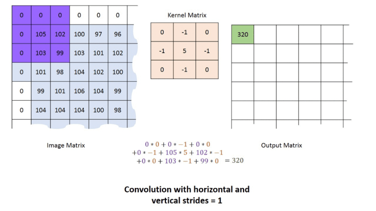
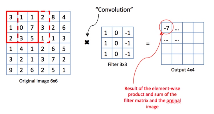
Let’s take a look. Consider the example above.
We have an image, and two alien terms: Kernel Matrix or Filter as it is referred to in image processing theory, and Output Matrix.
Both terms need some explanation but we’ll come to it later.
For now, let us understand the concept of convolution.
We start in the upper lefthand corner by placing the lefthand corner of filter on the underlying image and taking a dot product as shown in the graphic above. We then move the filter across the image step by step until it reaches the upper righthand corner. The size of the step is known as stride. Stride is a hyperparameter because we can move the filter to the right one column at a time, or we can choose to take larger steps. At each step, we take another dot product, and we place the results of that dot product in a third matrix, the output matrix or the activation map, the first alien term.
This is shown in the preceding graphic along with the calculations involved.
Although we have shown only one channel for illustration purposes, the filter actually applies to each channel (RGB) of our image.
Right. Back to the remaining alien term then.
This is the key that makes Convolutional Neural Networks so efficient. The job of the kernel matrix or filter is to find patterns in the image pixels in the form of features that can then be used for classification. What do we mean by ‘features’ and how can a mere 3×3 matrix be used to generate them? As we say, the best way to learn is by example.
Consider that we want to make a simple system that can classify the English alphabet. Let us use a 3×3 matrix as defined below. On convolving this with an image of letters E and A, we get the following result:

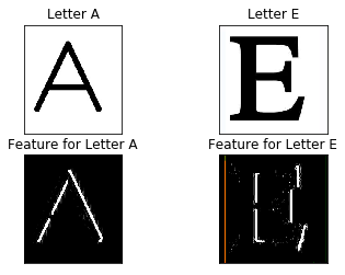
Intuitively, we can manually configure the system to classify letter A on basis of diagonal lines and letter E on the basis of vertical lines which are the features.
Right away we notice that in the previous case, we have defined the filter manually based on our knowledge.
But what if the system were able to learn this filter all by itself?
This is the fundamental concept of a Convolutional Neural Network.
It is the self-learning of such adequate classification filters, which is the goal of a Convolutional Neural Network.
We now come to the final part of this blog, which is the implementation of a CovNet using Keras. The reasons for using Keras have been discussed in the previous article.
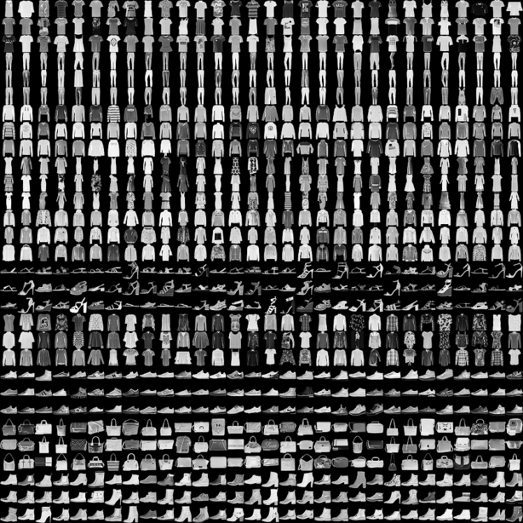
Since we can pride ourself on coming to the next level in AI computer vision algorithms, the dataset we will use is the Fashion MNIST because it is intended as a level up to the classic MNIST dataset, which we described as the “Hello, World” of machine learning programs that we used for Deep Neural Network in the previous article.
Just as the MNIST dataset contained images of handwritten digits, and Fashion MNIST contains, in an identical format, articles of clothing.
We will use 60,000 images to train the network and 10,000 images to evaluate how accurately the network learned to classify images.
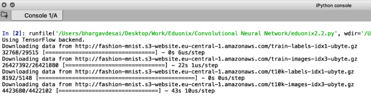
We can access the Fashion MNIST directly from Keras, just import the required libraries and then load the data:
import numpy as np import tensorflow as tf import keras from keras.models import Model from keras.models import Sequential, load_model from keras.layers import Dense, Conv2D, Dropout, Flatten, MaxPooling2D from keras.utils import np_utils fashion_mnist = keras.datasets.fashion_mnist (train_images, train_labels), (test_images, test_labels) = fashion_mnist.load_data()
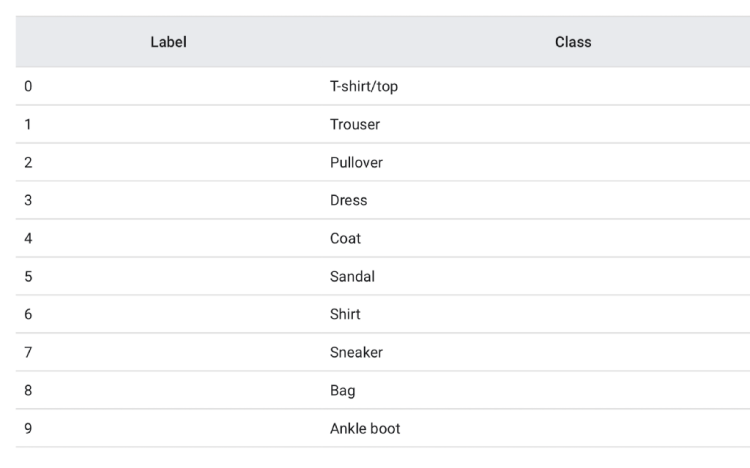
The train_images and train_labels arrays together are the training set which we will use to train the network and the test_images and test_labels arrays are on which we will evaluate the performance of our model. The labels and their classes are given as follows:
The shape of the training and test sets can be verified by:
train_images.shape Out[3]: (60000, 28, 28) test_images.shape Out[4]: (10000, 28, 28)
It is always better to visualize data for a quick sanity check. Let’s do that. We will plot the first 25 images with their class labels. The code for this is pretty straightforward.
import matlplotli.plyplot as plt plt.figure() for i in range(25): plt.subplot(5,5,i+1) plt.xticks([]) plt.yticks([]) plt.grid(False) plt.imshow(train_images[i], cmap=plt.cm.binary) plt.xlabel([train_labels[i]]) plt.show()
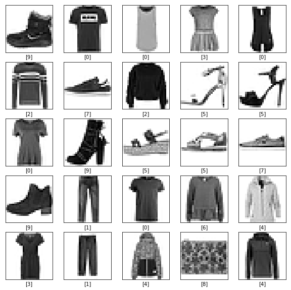
We encourage you to play around with the plt.xticks([]), plt.yticks([]), plt.grid(False) commands and see how the output changes.
A model is nothing but a stack of layers. Focus your attention on the libraries that we imported at the very beginning. Specifically the line:
from keras.layers import Dense, Conv2D, Dropout, Flatten, MaxPooling2D
Let’s go over these layers one by one quickly before we build our final model.
i. Dense: A Dense layer is just a bunch of neurons connected to every other neuron. Basically, our conventional layer in a Deep Neural Network.
ii. Conv2D: This is the distinguishing layer of a CovNet. This is a layer that consists of a set of “filters” which take a subset of the input data at a time, but are applied across the full input, by sweeping over the input as we discuss above. The operations performed by this layer are linear multiplications of the manner that we learned about prior. Keras allows us to define the number of filters along with their size and the stride.
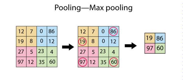
iii. MaxPooling2D: This layer simply replaces each patch in the input with a single output, which is the maximum (can also be average) of the input patch. This is best understood with a diagram:
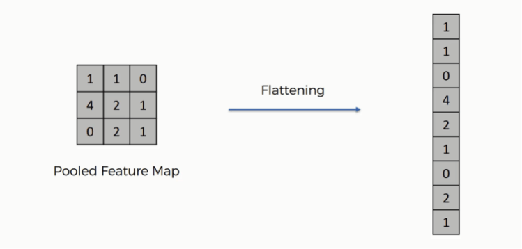
iv. Flatten: This layer just performs an ‘unroll’ operation on an activation map or output matrix so that we can pass it to a Dense layer. Again, let us understand this with an example:
In addition to the layers we have defined above, there is one more layer that is important called the Batch Normalisation Layer which normalizes the activations of each layer, consequently speeding up training.
Finally, our model. If you’ve read the previous blog in this Keras series, you would know that we always start defining our Keras model with the following line of code:
model = Sequential()
This creates a ‘Keras Model’ object, details of which you do not really have to worry about now.
We can now starting building our model by simply ‘adding’ layers to the Model object by model.add(…)
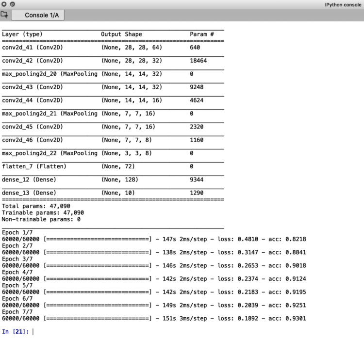
model.add(Conv2D(64, (3, 3), padding="same", activation='relu', input_shape=(28,28,1))) model.add(Conv2D(32, (3, 3), padding="same", activation='relu')) model.add(MaxPooling2D(pool_size=(2, 2))) model.add(Conv2D(32, (3, 3), padding="same", activation='relu')) model.add(Conv2D(16, (3, 3), padding="same")) model.add(MaxPooling2D(pool_size=(2, 2))) model.add(Conv2D(16, (3, 3), padding="same")) model.add(Conv2D(8, (3, 3), padding="same")) model.add(MaxPooling2D(pool_size=(2, 2))) model.add(Flatten()) model.add(Dense(128), activation = 'relu') model.add(Dense(10), activation = 'softmax') model.summary()
Note that the number of neurons in the last dense layer will always be equal to the number of classes we have, which in our case is 10.
Let us go over one of the code lines so that the meaning of this entire model building segment is intuitively clear.
We have mentioned previously that we can define the number of filters as well as the stride of a convolution layer in Keras.
model.add(Conv2D(64, (3, 3), padding="same", activation='relu', input_shape=(28,28,)))
Here, the first parameter inside the inner parenthesis, 64, defines the number of filters. The next parenthesis (3,3) defines the filter size. The parameter, padding=”same”, requires a bit of additional explanation.
We know from our knowledge of convolution that normally the filter moves covers the entire area in strides from one edge of the image to the other edge.
But there’s a problem here.
When moving the filter this way we see that the pixels on the edges are “touched” less by the filter than the pixels within the image. That means we are throwing away some information related to those positions. Furthermore, the output image is shrinking on every convolution, which could be intentional, but if the input image is small, we quickly shrink it too fast which may result in poor feature extraction and hence poor image classification accuracy.
A solution is a use of “padding”. Before we apply a convolution, we pad the image with zeros all around its border to allow the filter to slide on top and maintain the output size equal to the input. The result of padding in the previous example will be:
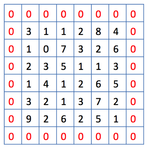
This is what is meant by the padding=”same” parameter.
The input shape is self-explanatory since the size of our images is 28 x 28.
Before moving on to compile our model, we will normalize our images between 0 and 1 to avoiding vanishing and exploding gradients during network training to increase stability.
We will also one-hot vectorize our training and test labels. The code for this is given below and the reason for these processes are described in greater detail in the previous blog of this series:
train_images = train_images/255.0 test_images = test_images/255.0 train_images = train_images.reshape(60000,28,28,1) test_images = test_images.reshape(10000,28,28,1) train_labels = np_utils.to_categorical(train_labels, 10) test_labels = np_utils.to_categorical(test_labels, 10)
We need to reshape the train_images and test_images the way shown otherwise, Keras will throw your dimensionality errors.
Compiling and training the model in Keras is done in two lines: model.compile(optimizer='adam', loss='categorical_crossentropy', metrics=['accuracy']) model.fit(train_images, train_labels, batch_size=32, epochs=7) model.save('simple_cnn_with_keras.h5') del model
The output screen should look something like this:
We conclude this blog on Convolutional Neural Networks by testing the model we have trained:
cnn_model = load_model('simple_cnn_with_keras.h5') accuracy_loss = cnn_model.evaluate(test_images, test_labels, verbose=2) print("Test Loss", accuracy_loss[0]) print("Test Accuracy", accuracy_loss[1])
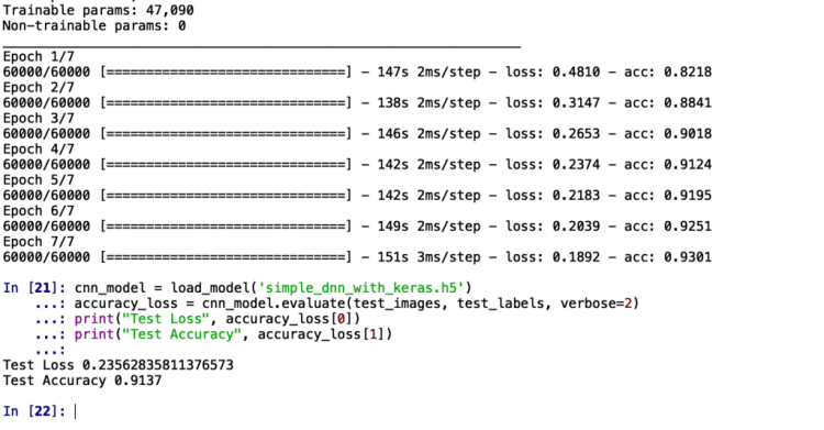
The accuracy we get on unseen images is 91.37%. This means out of the 10,000 images, we got classified 9,137 images correctly! Pretty neat, we’d say!

As a parting challenge, we’d like you to work on the same Dataset and see if you can match this accuracy by a Deep Neural Network discussed in the previous article!
Hit the comment section below with your results!
Let the battle of accuracies begin!


Convolutional Neural Networks with Keras was originally published in Becoming Human: Artificial Intelligence Magazine on Medium, where people are continuing the conversation by highlighting and responding to this story.

Have you ever wondered what goes into a creative mind? Creativity, especially artistic creativity, has long been considered innately human. But to what extent can deep learning be used to produce creative work, and how does it differ from human creativity?
As my first attempt in such exploration, I’d like the train an LSTM (long-short term memory) neural network on a set of jazz standards and generate new jazz music.
I wrote a scraper to download over 100 royalty-free jazz standards in MIDI format. MIDI files are more compact than MP3s and contain information such as the sequence of notes, instruments, key signature, and tempo, which makes processing music data easier.
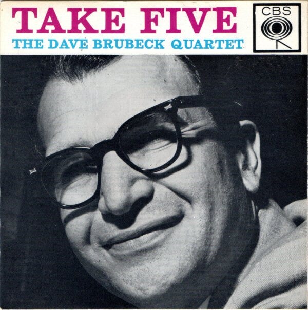
I selected a subset of songs to be my training dataset, including Dave Brubeck Quartet’s 1959 recording “Take 5”, one of the most requested and most popular songs of all time.
To extract data from MIDI files, I’m using music21, a python toolkit developed by MIT. I’m also using Keras, a deep-learning API that runs on top of Tensorflow, a library for deep neural networks.
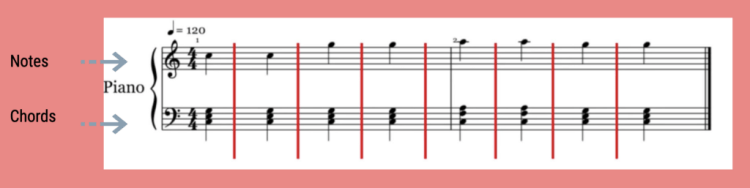
Generally speaking, there are three components to any given piece of music, melody, harmony, and rhythm. So for each MIDI file, I’m going to extract a sequence of notes, which represents melody, and chords, which represents harmony.
2. Generating neural speech synthesis voice acting using xVASynth
Similar to text data, music data is also sequential, thus a recurrent neural network (RNN) is used as the sequence learning model. In a nutshell, an RNN repeats the same operation over and over again, hence recurrent.
In particular, I will be using Long Short-Term Memory (LSTM) network, a type of RNN, which remembers information for a long period of time, typically used for text generation, or on time series prediction.
I’m setting the sequence length as 100, which means the next note is predicted based on the information from the previous 100 notes. Offset is the interval between two notes or two chords, so setting a number prevents notes from stacking. With those hyperparameters tuned, the model generates a list of notes, from which I can pick a random starting place, and I’m going to generate a sequence of 500 notes, which is the equivalent of about 2 mins of music, enough time to validate the quality of the output.
With everything said, here’s a snippet of the generated music:
Despite the fact that it sounds nothing like what a jazz musician would play, I’m impressed by the fact that there are a variety of melodic elements and somewhat jazz harmony. The rhythm can most definitely be improved.
This concludes my personal attempt at training a music generation model. As far as AI-music creation goes, there’s Google’s Magenta project which produced songs written and performed by AI, and Sony’s Flow Machines has released a song called “Daddy’s Car” based on the music of The Beatles.
With potentially more complex models, there is a lot neural networks can do in the field of creative work. While AI is no replacement for human creativity, it’s easy to see a collaborative future between artists, data scientists, programmers, and researchers to create more compelling content.
The code for this project can be found on my GitHub page. Feel free to reach out and connect with me here or on LinkedIn. Thanks!
Generating Music Using LSTM Neural Network was originally published in Becoming Human: Artificial Intelligence Magazine on Medium, where people are continuing the conversation by highlighting and responding to this story.

Correctly applying the hypothesis testing process is extremely essential for drawing out valid A/B testing conclusions. In this post, I have explained the statistical concepts behind conducting a successful A/B test.
A hypothesis is a simple, testable statement that helps compare the two variants. The assumption of a statistical test is called the Null Hypothesis (H0) and a violation of that assumption is called the alternative hypothesis (H1). The null hypothesis is often called the default assumption, or the assumption that nothing has changed. The testing procedure begins with the assumption that the null hypothesis is true. For instance, if you’re conducting an A/B test to know whether the color change that you made to your website resulted in a higher end of visit conversion rate or not, your null hypothesis would state that the change had no effect on the conversion rate.
To lay down a well-formed hypothesis, include the following parameters in your statement.
a) Population (who is being affected by the change?)
b) Intervention (what change are you testing?)
c) Comparison (what are you comparing it against?)
d) Result (what is the resulting metric that you’re measuring?)
e) Time (when are you measuring the resulting metric?)
In the previous example, a well-formed hypothesis would be:
H0: Website X visitors (population) who visit the page with the change in color (Intervention) will not have higher end of visit (Time) conversion rates (Result) when compared to visitors who visit the default page.
H1: Website X visitors who visit the page with the change in color will have higher end of visit conversion rates when compared to visitors who visit the default page.
A statistical hypothesis test may return a value called the p-value. This is the value used to interpret the statistical significance of the test. The p-value is used in either rejecting the null hypothesis or in failing to reject the null hypothesis. This is done by comparing the p-value to a threshold value called the significance level which is set before starting the experiment. The significance level (alpha or Type 1 error) is usually set at 5% or 0.05. The value of alpha depends upon the business scenario and the cost associated with Type I and Type II errors.
The textbook definition of p-value is the probability that the result would be as extreme as the one computed/observed given that the null hypothesis is true. In simpler terms, the p-value can be seen as the probability of getting the observed result simply by chance. For example, if we observed a p-value of 0.02 for our scenario, then we can say that the probability of observing the higher conversion rate (say X %) for the treatment group (visitors who received the page with the color change) by chance is just 2%. Since this p-value is less than the significance level, we reject the Null hypothesis and state that the color change indeed resulted in a higher conversion rate than the default page.
While conducting A/B tests, the two types of errors you should care about are Type I and Type II errors. Type I error is the probability of rejecting the null hypothesis when it is true and Type II error is the probability of failing to reject the null hypothesis when it is false.
The type II error is represented by the symbol β. The Statistical power is then defined as the inverse of that i.e. 1- β. So, if the type II error is 0.1 or 10% then the statistical power of that test is 0.9 or 90% (1–0.1=0.9).
2. Generating neural speech synthesis voice acting using xVASynth
The statistical power of a test depends on 3 parameters of the design of an A/B test: the minimum effect size of interest, the significance level (or alpha) set as a threshold, and the sample size.
a. Higher the significance level, lower is the statistical power, given that all other factors are constant.
b. Lower the minimum effect of interest, lower is the statistical power, given that all other factors are constant.
c. Larger the sample size, the higher the statistical power, given that all other factors are constant.
Choosing an adequate level of statistical power is highly important while designing an A/B test in order to avoid wasting resources.
In your A/B test, after determining whether the variant had an impact or not, it is also important to measure how much the impact is. The effect size is the absolute difference between the two groups’ resultant metrics (the conversion rates in our case). It can either be expressed in percentage points or in terms of standard deviation.
Estimating the effect size at the start of the test helps in determining the sample size and the statistical power of the test.
Confidence intervals give the range of values where the resultant/observed metric will probably be found. You would need to construct separate confidence intervals for the resultant metric for both the control and the treatment group. For our example, we could say that We are 95% confident that the true conversion rate for the colored page is X% +/- 3%. The 3% here is the margin of error.
One thing to keep in mind is that if the 95% confidence level for the control group’s conversion rate overlaps with the 95% confidence level for the treatment group’s conversion rate, then you would need to keep testing to arrive at a statistically significant result.
References
1] B.Michael, Data Science You Need to Know(2018), Towards Data Science
Statistical Concepts behind A/B Testing was originally published in Becoming Human: Artificial Intelligence Magazine on Medium, where people are continuing the conversation by highlighting and responding to this story.
Originally from KDnuggets https://ift.tt/2ZFO63J
Originally from KDnuggets https://ift.tt/3dBjrg4
Originally from KDnuggets https://ift.tt/3pRzBod
Originally from KDnuggets https://ift.tt/3sfxz2C
