365 Data Science

Tales of an oceanographer navigating the different waves of tech companies looking for whales.

1. Introduction and Hypothesis

I loved to work as a scientist. There is a deep feeling of completion and happiness when you manage to answer why. Finding out why such animal would go there, why would they do this at that time of the year, why is that place so diverse… This applies to any kind of field. This is the reason why I want to advocate that if you are a scientist, you might want to have a look at what is called Data Science in the technological field. Be aware, I will not dwell in the details of titles such as Data engineer, data analyst, data scientist, AI researcher. Here, when I refer to Data Science, I mean the science of finding insights from data collected about a subject.

So, back to our why. In science, in order to answer your why, you will introduce the whole context surrounding it and then formulate an hypothesis. “The timing of the diapause in copepods is regulated through their respiration, ammonia excretion and water column temperature”. Behaviour of subject is the result of internal and external processes.
In marketing, you would have to formulate similar hypothesis in order to start your investigation: “3-days old users un-suscribes due to the lack of direct path towards the check-out”. Behaviour of subject is the result of internal (frustration) and external (not optimized UE/UI) processes.

• References

Although I would have wanted to put that part at the end, as for any scientific paper, it goes without saying that your introduction would present the current ideas, results, and hypotheses of your field of research. So, as a researcher, you need to accumulate knowledge about your subject, and you go looking for scientific articles. The same is true for techs as well. There are plenty of scientific and non-scientific resources out-there that will allow you to better understand, interpret and improve your product. Take this article, for instance, Medium is a wonderful base of knowledge on so many topics! But you could also find passionating articles on PloS One on Users Experience or Marketing Design and etc.

2. Material and Methods

• Data collection

As a Marine biologist and later an Oceanographer, I took great pleasure to go at the field and collect data (platyhelminths, fish counts, zooplankton , etc..). Then we needed to translate the living “data” into numeric data. In the technological industry, it is the same idea. Instead of nets, quadrats, and terrain coverage, you will setup tracking event, collect postbacks from your partners and pull third-parties data. The idea is the same, “how do I get the information that will help me answer my why”. So a field sampling mission and a data collection planning have a lot in common.

Trending AI Articles:

1.Write Your First AI Project in 15 Minutes

2. Generating neural speech synthesis voice acting using xVASynth

3. Top 5 Artificial Intelligence (AI) Trends for 2021

4. Why You’re Using Spotify Wrong

• Data treatment

In ecology and oceanography, you need to have the big picture. You play with a lot of scales (spatial, temporal). And to do so, you usually want to have the most complete dataset possible. So you interpolate missing data, you decide to remove some of it or you resample (when you have the time and fundings). This is exactly what you also do in the technologies industry: In order to better understand your product, you want to know as much as you can, so you setup tracking event, you record your demography through google analytics and you aggregate your raw data into “cooked” data with AWS Lambda. Although all of this may sound alien to you if you are from academia, this is pretty much the same idea behind field sample and then identification of you species and environmental variables.

• Language used

-SQL is a must have

As an advice, if you which to become a data analyst or a data scientist, I strongly advice to learn about SQL. When I was studying my evolution courses using R, it was such a pain to have to select specific data from that column where the value of this other column was equal to pink… When I started using SQL, it made so much sense. With your “mind” representation of your data, SQL is a declarative language where you can get multiple parameters while using multiple “WHERE” clauses. Some of them even use parallelization technologies (Hadoop) to get your data event faster (MySQL to site one).

-Python for all

Then, once you have your data, you can play with it. This is where you can clean it, join it with other data or aggregate it into different data using formulas. Python is one of the best language for that as it is really simple to understand. From someone who spent his whole academia life using R, MatLab (and Ferret), it took me maybe 2 months to be comfortable using Python and maybe 6 months to be completely autonomous (although it never hurts to have your code reviewed).

3. Results and Interpretation

Once you understand your data, that you have the full picture (or at least the closer vulgarization of what the truth would be), we want to share our findings with our peers. In science, we do so by the mean of presentations in symposium or scientific papers. Of course we could have feedbacks from our supervisor or reviewers, but they usually take ages to come and they are also mostly a one-way discussion. Meanwhile in tech, you will have to present your findings to people that do not have the same background as you do. Being excited about using that specific statistical technique of clustering because it was the exact use case (nope, that never happened to me…) will not make them as excited as you are.

You will need to work on what is the core take away from your findings.

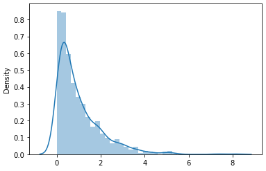
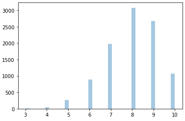
That essentialist approach led me to make very simple figures with at the most 2 metrics in them. Then I had to present in person the results which led me to work on how to express myself for a more general audience.

With a simple approach, I realized also that I needed to look at the simple questions first, the “quick wins” as they say, that would then lead me towards more detailed analysis.

Of course, all of the above points can be found in academia, but in the tech industry, you have to do some studies from the ground up every month (sometimes every week depending on the project). In academia, you are the expert of your field, but you only focus on it and rarely venture elsewhere. You may have a couple of presentations a year and at most you are working on 1 to 3 paper a year. In the tech industry, you have reports to give every week. One day you can work on the acquisition cohorts of Whales (high-spending users) and the next you have to create a forecasting function that will identify potential users that will churn (un-subscribe/cancel or leave the product). The presentations are every month or even every week. So yeah, the pace is much more dynamic in the tech industry but also, you learn so much more, faster.

I know there are a lot of us who spent quite some times in academia who could not pursue it. Whether it was because your supervisor had a different agenda, you were sick of struggling to be able to afford a decent life or that there were no opportunities where you lived, it is not the end of the world. I found all the things that I loved in science in the tech industry. Flexible hours, creating your own projects, being responsible for your budget (in time) and sampling tools (homemade functions, third-parties solutions), the thrill of the investigation, and, in the end, presenting your results to your peers and have feedback on the spot that will lead to further studies.

In the meantime, nothing stops you from volunteering in an association. I realized that I had a better impact on the planet working in a marketing company but volunteering at picking trash while running in the forest than doing Arctic bio-geo-chemical modeling… So, do not hesitate to take a leap of faith, you have nothing to lose and only all to gain.

Don’t forget to give us your ? !

---

From Science to Data Science was originally published in Becoming Human: Artificial Intelligence Magazine on Medium, where people are continuing the conversation by highlighting and responding to this story.

Via https://becominghuman.ai/from-science-to-data-science-8e683fde3312?source=rss—-5e5bef33608a—4

Statistical Distributions!

The normal distribution is the most important probability distribution in statistics because it fits many natural phenomena.

In this article we will cover some distributions that I have found useful while analysing data. I have split them based on whether they are for a continuous or a discrete random variable. First I give a small theoretical introduction about the distribution, its probability density function, and then how to use python to represent it graphically.

Continuous Distributions:

• Uniform distribution
• Normal Distribution, also known as Gaussian distribution
• Standard Normal Distribution — case of normal distribution where loc or mean = 0 and scale or sd = 1
• Gamma distribution — exponential, chi-squared, erlang distributions are special cases of the gamma distribution
• Erlang distribution — special form of Gamma distribution when a is an integer ?
• Exponential distribution — special form of Gamma distribution with a=1
• Lognormal — not covered
• Chi-Squared — not covered
• Weibull — not covered
• t Distribution — not covered
• F Distribution — not covered

Discrete Distributions:

• Poisson distribution is a limiting case of a binomial distribution under the following conditions: n tends to infinity, p tends to zero and np is finite
• Binomial Distribution
• Negative Binomial — not covered
• Bernoulli Distribution is a special case of the binomial distribution where a single trial is conducted n=1
• Geometric — not covered

Lets import some basic libraries that we will be using:

import numpy as np
import pandas as pd
import scipy.stats as spss
import plotly.express as px
import seaborn as sns

Trending AI Articles:

1.Write Your First AI Project in 15 Minutes

2. Generating neural speech synthesis voice acting using xVASynth

3. Top 5 Artificial Intelligence (AI) Trends for 2021

4. Why You’re Using Spotify Wrong

Continuous Distributions

Uniform distribution

As the name suggests, in uniform distribution the probability of all outcomes is same. The shape of this distribution is a rectange. Now, lets plot this using python. First we will generate an array of random variables using scipy. We will specifically use scipy.stats.uniform.rvs function with following three inputs:

• size specifies number of random variates
• loc corresponds to mean
• scale corresponds to standard deviation

rv_array = spss.uniform.rvs(size=10000, loc = 10, scale=20)

Now we can plot this using the plotly library or the seaborn library. Infact seaborn has a couple of different function, namely the distplot and the histplot, both of which can be used to visually view the unoform data. Lets see the examples one by one:

We can directly plot the data from the array:

px.histogram(rv_array) # plotted using plotly express
sns.histplot(rv_array, kde=True) # plotted using seaborn

Or we can convert array into a dataframe and then plot the data frame:

rv_df = pd.DataFrame(rv_array, columns=['value_of_random_variable'])

px.histogram(rv_df, x='value_of_random_variable', nbins=20) # plotted using plotly express

sns.histplot(data=rv_df, x='value_of_random_variable', kde=True) # plotted using seaborn

Normal Distribution, also known as Gaussian distribution:

The normal distribution is the most important probability distribution in statistics because it fits many natural phenomena. Normal distribution is a limiting case of Poisson distribution with the parameter lambda tends to infinity. Additionally since poisson distribution is a for of binomial distribution, normal distribution is also a form of binomial distribution. This distribution has a bell-shaped density curve described by its mean and standard deviation. The mean represents the location and the sd represents the spread of the distribution. The curve represents that the data near the mean occurrs more frequently than the data far from the mean.

Lets plot it using seaborn:

rv_array = spss.norm.rvs(size=10000,loc=10,scale=100)  # size specifies number of random variates, loc corresponds to mean, scale corresponds to standard deviation

sns.histplot(rv_array, kde=True) 

We can add x and y labels, change the number of bins, color of bars, etc. With distplot we can supply additional arguments for adjusting width of bars, transparency, etc.

ax = sns.distplot(rv_array, bins=100, kde=True, color='cornflowerblue', hist_kws={"linewidth": 15,'alpha':1})

ax.set(xlabel='Normal Distribution', ylabel='Frequency')

Standard Normal Distribution

Is a special case of the normal distribution where mean = 0 and sd = 1

Lets plot it using seaborn:

rv_array = spss.norm.rvs(size=10000,loc=0,scale=1) 

sns.histplot(rv_array, kde=True)

Gamma distribution is a two-parameter family of continuous probability distributions

Exponential, chi-squared, erlang distributions are special cases of the gamma distribution

Lets plot it using seaborn:

rv_array = spss.gamma.rvs(a=5, size=10000) # size specifies number of random variates, a is the shape parameter

sns.distplot(rv_array, kde=True)

Erlang distribution

Special case of Gamma distribution when a is an integer.

Exponential distribution

Special case of Gamma distribution with a=1. Exponential distribution describes the time between events in a Poisson point process, i.e., a process in which events occur continuously and independently at a constant average rate.

Lets plot it using seaborn:

rv_array = spss.expon.rvs(scale=1,loc=0,size=1000) # size specifies number of random variates, loc corresponds to mean, scale corresponds to standard deviation

sns.distplot(rv_array, kde=True)

Discrete Distributions

Binomial Distribution

Distribution where only two outcomes are possible, such as success or failure, gain or loss, win or lose. Additionally, the probability of success and failure is same for all the trials. Further, the outcomes need not be equally likely, and each trial is independent of each other.

The probability of observing k events in an interval is given by the equation: f(k;n,p) = nCk * (p^k) * ((1-p)^(n-k)) Where, nCk = (n)! / ((k)! * (n-k)!) n=total number of trials p=probability of success in each trial

Lets plot it using seaborn:

rv_array = spss.binom.rvs(n=10,p=0.8,size=10000) # n = number of trials, p = probability of success, size = number of times to repeat the trials

sns.distplot(rv_array, kde=True)

Poisson Distribution

Poisson random variable is typically used to model the number of times an event happened in a time interval. For example, the number of users registered for a web service in an interval can be thought of as a Poisson process. Poisson distribution is described in terms of the rate (μ) at which the events happen. The average number of events in an interval is designated λ (lambda). Lambda is the event rate, also called the rate parameter. The probability of observing k events in an interval is given by the equation: P(k events in interval) = e^(-lambda) * (lambda^k / k!)

Poisson distribution is a limiting case of a binomial distribution under the following conditions:

• The number of trials is indefinitely large or n tends to infinity
• The probability of success for each trial is same and indefinitely small or p tends to zero
• np = lambda, is finite.

Lets plot it using seaborn:

rv_array = spss.poisson.rvs(mu=3, size=10000) # size specifies number of random variates, loc corresponds to mean, scale corresponds to standard deviation

sns.distplot(rv_array, kde=True)

Bernoulli distribution

This distribution has only two possible outcomes, 1 (success) and 0 (failure), and a single trial, for example, a coin toss. The random variable X which has a Bernoulli distribution can take value 1 with the probability of success, p, and the value 0 with the probability of failure, q or 1-p. The probabilities of success and failure need not be equally likely. Probability mass function of Bernoulli distribution: f(k;p) = (p^k) * ((1-p)^(1-k))

Bernoulli distribution is a special case of the binomial distribution where a single trial is conducted (n=1)

Lets plot it using seaborn:

rv_array = spss.bernoulli.rvs(size=10000,p=0.6) # p = probability of success, size = number of times to repeat the trial

sns.distplot(rv_array, kde=True)

Hope you found this summary of distributions useful. I refer to this from time to time to jog my memory on the various distributions.

Comments welcome!

Don’t forget to give us your ? !

---

Statistical Distributions was originally published in Becoming Human: Artificial Intelligence Magazine on Medium, where people are continuing the conversation by highlighting and responding to this story.

Via https://becominghuman.ai/statistical-distributions-533260f370f2?source=rss—-5e5bef33608a—4

The rapid development of Transformers have brought a new wave of powerful tools to natural language processing. These models are large and very expensive to train, so pre-trained versions are shared and leveraged by researchers and practitioners. Hugging Face offers a wide variety of pre-trained transformers as open-source libraries, and you can incorporate these with only one line of code.

Originally from KDnuggets https://ift.tt/2ZlwwBP

We’re excited to announce that a new open-source project has joined the Alteryx open-source ecosystem. EvalML is a library for automated machine learning (AutoML) and model understanding, written in Python.

Originally from KDnuggets https://ift.tt/3s4JPDb

Using continual learning might avoid the famous catastrophic forgetting problem in neural networks.

Originally from KDnuggets https://ift.tt/37jcRH1

As more people are entering the field of Data Science and more companies are hiring for data-centric roles, what type of jobs are currently in highest demand? There is so much data in the world, and it just keeps flooding in, it now looks like companies are targeting those who can engineer that data more than those who can only model the data.

Originally from KDnuggets https://ift.tt/3ptMe8M

Also: The Best Data Science Project to Have in Your Portfolio; How to Get Your First Job in Data Science without Any Work Experience; How to Get Data Science Interviews: Finding Jobs, Reaching Gatekeepers, and Getting Referrals

Originally from KDnuggets https://ift.tt/3b6lHsW

Pick your visualizations strategically. They need to tell a story.

Originally from KDnuggets https://ift.tt/3jQwmvz

Linear algebra is the branch of mathematics that studies vector spaces. You’ll see how vectors constitute vector spaces and how linear algebra applies linear transformations to these spaces. You’ll also learn the powerful relationship between sets of linear equations and vector equations.

Originally from KDnuggets https://ift.tt/37aZZCV

Deep Learning in Self-Driving Cars

The very first self-driving car used Neural Networks to detect lane lines, segment the ground, and drive. It was called ALVINN and was created in 1989.

Great Scott! Neural Networks were already used back in 1989! The approach was End-To-End: you feed an image to a neural network that generates a steering angle. Et voila.

In 2021, it’s even crazier. Deep Learning has taken over the major subfields of autonomous driving.

In this article, I’d like to show you how Deep Learning is used, and where exactly.

In order to do this, I will go through all 4 pillars of autonomous driving, and explain how Deep Learning is used there.

In a few words:

• In Perception, you find the environment and obstacles around you.
• In Localization, you define your position in the world at 1–3 cm accuracy.
• In Planning, you define a trajectory from A to B, using perception and localization.
• In Control, you follow the trajectory by generating a steering angle and an acceleration value.

? If you’re a complete self-driving car beginner, I recommend you check my series of articles on these 4 topics.

In this article, you will learn how Deep Learning is implemented on all 4 modules, and if you’re aspiring to work on self-driving cars, which skills you need to learn to be a Deep Learning Engineer.

For that, I will use a MindMap and link you to recorded videos. At the end of this article, I’ll give you the link to download this MindMap, and an Autonomous Tech Starter Kit.

Before we start, I’m running a Daily Mailing List on self-driving cars & cutting-edge technologies, and I’d love to have you with us!

Deep Learning in Perception

Perception is the first pillar of autonomous driving, and as you may have guessed, there is a lot of Deep Learning involved. Every student going through his first Deep Learning course will hear “Deep Learning is used in self-driving cars to find the obstacles or the lane lines”.
These applications belong to Perception.

Perception generally uses 3 sensors:

• The Camera
• The LiDAR (Light Detection and Ranging)
• The RADAR (Radio Detection and Ranging)

To understand better these 3 sensors, you can check the introduction of my Sensor Fusion article.

Trending AI Articles:

1. Write Your First AI Project in 15 Minutes

2. Generating neural speech synthesis voice acting using xVASynth

3. Top 5 Artificial Intelligence (AI) Trends for 2021

4. Why You’re Using Spotify Wrong

Camera Detection

In the following graph, I show the most significant use cases, how they’re implemented, and how to learn to implement it yourself.

• In light yellow, you will see how to solve the tasks using traditional techniques.
• In dark yellow, you will see how to solve the tasks using Deep Learning.
• In blue, these are online course recommendations if you want to learn.

As you can see, Computer Vision is requiring a lot of Deep Learning for the task of detection.

In Lane Line Detection and Segmentation, we use Deep Learning over traditional techniques because they’re faster and more efficient. Algorithms such as LaneNet are quite popular in the field of research to extract lane lines. ? To learn more about it, you can also check my article on Computer Vision.

2D Object Detection is also at the heart of Perception. Algorithms such as YOLO or SSD have been very well explained and are very popular in this field. They’re constantly updated, replaced with new ones, but the idea is similar.
? If you’d like to learn more, here’s my research review on YOLOv4.

Finally, many camera setups are made in Stereo.
Having Stereo information helps us build what’s called a Pseudo-LiDAR. We can completely emulate and even sometimes replace the LiDAR, and therefore do 3D Perception with cameras (2D sensors).

For that, we used to implement Block Matching using traditional Computer Vision… and we’re now switching to Deep Learning.
? My article on Pseudo-LiDARs and my course on 3D Computer Vision can help you understand more.

LiDAR Detection

First, traditional approaches based on the RANSAC algorithm, 3D Clustering, KD-Trees and other unsupervised learning techniques are still the go-to for many robotics applications.
? I teach these in my Point Cloud Fast Course if you’re interested.

However, these aim to be replaced by Deep Learning approaches, faster and safer. Why? Because naïve algorithms can’t classify, or tell that two very close people are indeed two people. A learning approach is more suited here.

Many object detection in 3D papers have been released by companies such as Apple  (VoxelNet), UBER ATG (PIXOR and Fast and Furious), nuTonomy (PointPillars), and the University of Oxford (RANDLANET).

At the heart of it, we find techniques such as 3D CNNs (Convolutional Neural Networks) or PointNet. These are the fundamentals of 3D Deep Learning.

These days, LiDAR detection using Deep Neural Networks is booming. That’s one of the most active area of research in self-driving cars.

RADAR Detection

RADAR is a very mature sensor. It’s over 100 years old, and it’s no shame to say it doesn’t need Deep Learning to be efficient. Using RADARs, we’ve been able to measure obstacles speed for decades. In fact, if you’ve got a speed ticket lately, it’s because of RADARs.
? The techniques used for this are well explained in my dedicated article.

Deep Learning in RADARs is starting to emerge with algorithms such as Centric 3D Obstacle Detection or RADAR Region Proposal Network. However, it seems to still be early research.

Sensor Fusion

The final part of Perception is Sensor Fusion.

To make the detection “sure”, we include what’s called redundancy. The idea is simple: we merge data from sensors and check if they tell the same thing.

There are 3 ways to merge for a company using all 3 sensors:

• Merging Camera and LiDAR
• Merging Camera and RADAR
• Merging LiDAR and RADAR

Here’s a map that shows you all the ways we use Deep Learning in Sensor Fusion.

Every time, I make the distinction between early and late fusion.

• Early Fusion means you’re fusing the raw data, such as LiDAR point clouds and Image pixels.
• Late Fusion means you’re fusing the output of the detections, such as a 2D and a 3D Bounding Box.

What’s interesting is that Deep Learning is more or less suited depending on the sensor used.

? For LiDAR camera fusion, a process such as the one I’m explaining in this article is used as a traditional approach.
But Deep Learning starts to be very well suited for this process.
Since we handle Deep Learning well with the camera and LiDAR, it’s understandable why we use Deep Learning for the fusion of the two.

Since RADARs don’t use a lot of Deep Learning, it’s more complicated and you’ll find more approaches involving Kalman Filters, IOU matching and tracking.

Again, you can start to see the impact of Deep Learning in Sensor Fusion. The discipline is usually very traditional, uses a lot of robotics and bayesian filtering. It tends to use Computer Vision feature detectors rather than CNNs… and now, it’s transforming into a Deep Learning discipline.

I have a complete recap of Perception:

Deep Learning in Localization

Localization is about finding the position of the ego vehicle in the world.
The first thing that comes in mind is to use GPS, but you’ll find out it can be very inaccurate and might not work perfectly every time, for example when it’s cloudy.
In the end, GPS is accurate to 1–2m, while we’re targetting 1-3 cm.

This problem created a whole field we call localization.

Depending on the algorithmic choice, we have many ways to do localization:

Knowing the Map and the initial position

Imagine you’re in New York, on the 5th Avenue (I miss traveling?). And imagine you have a map of the Big Apple. Theorically, you just need to count how many steps you took in the streets to know where you’ll be after a 10 minutes walk. That’s the first case, you have the map (New York) and your position.

Knowing the Map, but not the initial position

Now imagine you’re still in New York, but you’ve been kidnapped, blindfolded, and placed somewhere else. You’ll need to use your eyes and knowledge of the map to determine your position. When you recognize something familiar such as the Empire State Building, you’ll know where you are!

These two things therefore rely on something we called landmark detection. We want to detect things we know and which are in the map.

To do this, we use Extended Kalman Filters and Particle Filters.
? The difference is explained in my article on Localization.

As you noticed, we’re also using Odometry (how much the wheels spin, GPS, GPS-RTK (a better GPS), and UWB (trilateration using physical devices).

If you’re looking for Deep Learning, there’s just the landmark detection, that is obtained in the Perception step.

Knowing neither the Map nor the initial position

Now imagine you’re kidnapped, blindfolded, and put somewhere in New York but you don’t have the map.

That’s called Simultaneous Localization And Mapping (SLAM): you need to both locate and build a map of your surroundings.

The SLAM field originally uses a lot of Bayesian Filtering, such as Kalman and Particle Filters, but something called Visual Odometry is currently booming.

The idea is to use sensors such as cameras, or stereo cameras, to recreate an environment and therefore a map. Here’s a map of SLAM, and you can also read this paper to understand it better.

As you can see, there is a lot of Deep Learning involved for mapping and localization… but the field is primarly not using Deep Learning. If you’d like to be a localization engineer, it’s much more important to have a great understanding of robotics and traditional techniques than Deep Learning.

The explanation of this Localization Mindmap is here:

Deep Learning in Planning

Planning is the brain of an autonomous vehicle. It goes from obstacle prediction to trajectory generation. At its core: Decision Making.

We can divide the Planning world in 3 steps:

• High-Level/Global Planning — Programming the route from A to B.
• Behavioral Planning — Predicting what other obstacles will do, and making decisions
• Path/Local Planning — Avoid obtacles, and create a trajectory.

To use Deep Learning in self-driving cars, the best way is to do Perception… but the second best way is through Planning.

High Level Planning

The first thing is to program a route from A to B, like Google Maps or Waze.
For that, we’ll have to use Graph Search algorithms such as Dijkstra, A*, DFS, BFS, …

Commonly, A* is used.

But you’ll also find a lot of Deep Reinforcement Learning here: that’s called Probabilistic Planning.

Behavioral Planning

This step includes 2 sub-steps:

• Prediction
• Decision-Making

In prediction, we want to use time information and data association to understand where an obstacle will be in the future. Learning-based approaches such as Gaussian Mixture Models for Intent Prediciton can be found… and Kalman Filters approaches too; as in my most popular article Computer Vision for Tracking.

Decision-Making is something different. We either manually input some rules and create a Finite State Machine, or we don’t, and use Reinforcement Learning approaches.

Path Planning

Global Planning is good to know where you’re supposed to go in a map. But what if a car is blocking? What if the traffic light is red? What is a vehicle is very slow? We need to do something, like modifying the trajectory, or stopping the car.

A lot of algorithms such as Rapidly-exploring Random Trees (RRT), RRT*, Probabilistic RoadMaps (PRM), PRM*, … are in use.

In planning, if we use Deep Learning, it can mostly be in Prediction, or Path Planning using Reinforcement Learning approaches.

Deep Learning in Control & Other Applications

Control

Control is, as said in the introduction, about following the generated trajectory by generating a steering angle and an acceleration value.

When I first searched to write this article, I thought “There is no Deep Learning in Control”. I was wrong.

As it turns out, Deep Reinforcement Learning is starting to emerge in both Planning and Control, as well as End-To-End approaches such as the one ALVINN used.

Other Applications

The 4 pillars of autonomous driving are somehow all using Deep Learning. However, there are many other ways Deep Learning can be used….

Explainable AI, GANs to generate synthetic datasets, Active Learning to have semi-automated labelling, and more…

Here’s the video on Control and the other use.

Conclusion

If you’ve read that far, congratulations! You’re much closer to understanding self-driving cars now that you were 10 minutes ago!

As you can see, Deep Learning is well in place in many areas of autonomous driving… and it’s emerging in all the others.

If you’re interested in self-driving cars & AI, I invite you to join the Mailing List on Self-Driving Cars, it gives access to a starter pack made of 4 fundamental resources, including this Deep Learning MindMap we just saw.

? Join the Daily Emails

Thank you for reading, and don’t forget to learn Deep Learning.

Jeremy Cohen

Don’t forget to give us your ? !

---

Deep Learning Algorithms in Self-Driving Cars was originally published in Becoming Human: Artificial Intelligence Magazine on Medium, where people are continuing the conversation by highlighting and responding to this story.

Via https://becominghuman.ai/deep-learning-algorithms-in-self-driving-cars-14b13a895068?source=rss—-5e5bef33608a—4