Today, cloud data storage accounts for 45% of all enterprise data and by Q2 2021, that number could grow to 53%. Now is the time to embrace cloud than now.
Originally from KDnuggets https://ift.tt/2K8jZxJ

365 Data Science is an online educational career website that offers the incredible opportunity to find your way into the data science world no matter your previous knowledge and experience.
Originally from KDnuggets https://ift.tt/2K8jZxJ
Originally from KDnuggets https://ift.tt/38z9IUz
Originally from KDnuggets https://ift.tt/35vtUVD

Generating Area Importance Heatmaps with Occlusions
Continue reading on Becoming Human: Artificial Intelligence Magazine »

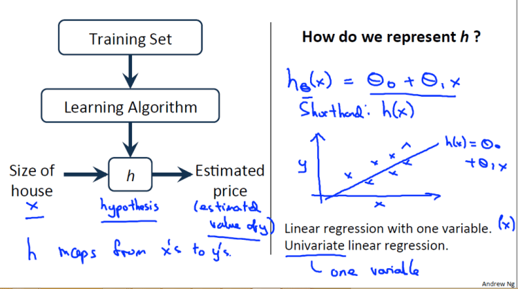
In general, linear regression is an approach to modelling the relationship between a dependent variable and independent variables. Linear regression is also consider as next step up after correlation. It is function to predict the dependent value of the output variable based on the value of another independent variable. Univariate and multivariate regression represent two approaches to statistical analysis. Univariate involves the analysis of a single variable while multivariate analysis examines two or more variables. Most multivariate analysis involves a dependent variable and multiple independent variables. In this short article, we will focus on univariate linear regression and determine the relationship between one independent (explanatory variable) variable and one dependent variable. For example, given training data including size of house and its respective price, we would like to predict the price based on size of house.
In this work, a linear regression algorithm is implemented without using machine learning library such as Scikit-Learn or TensorFlow. The dataset used in this simple experiment is obtained from Kaggle.
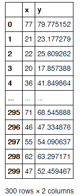
Using the given x and y point values, we will investigate the relationship between unit x and y. It is typical univariate regression case as it only consider one feature and one dependent variable. Although the relationship between x and y is obviously to be spotted, it is still a good example to demostrate the application of univariate linear regression.

Firstly, we have to import some of the essential libraries.
import numpy as np
import matplotlib.pyplot as plt
import seaborn as sns
import pandas as pd
The downloaded dataset file named fabricated_points.csv. It may vary for different users if they rename the file once downloaded.
data = pd.read_csv("fabricated_points.csv")
We assign the feature values and corresponding output values to X and Y arrays accordingly.
X = np.array(data['x']).reshape(-1,1)
Y = np.array(data['y']).reshape(-1,1)
The X array consists of values from x column and then reshape to 1 column as shown in below.

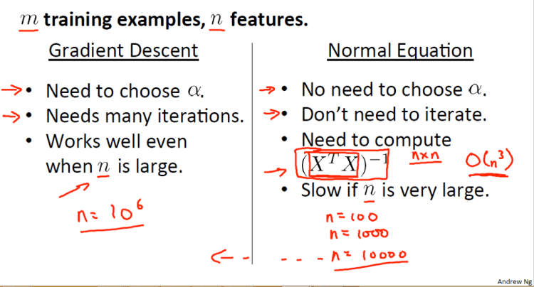
The motive in Linear Regression is to minimize the cost function. Before we build linear regression model from scratch, it will be great if we have someting to verify our model is working correctly. One of the method to determine the minimum cost value is Normal Equation. It is an analytical way to solve for weights (or called parameter) with a Least Square Cost Function.
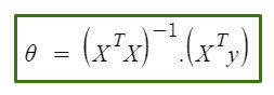
We can directly find out the value of θ without using Gradient Descent, the θ value is then mutiply with X input, it should give the respective Y values. It is time-saving method. However, it only effective for small features data.
ne_theta = np.linalg.inv(X.T.dot(X)).dot(X.T).dot(Y)
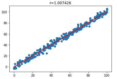
The ne_theta, θ value is 1.0074256. We can scatter the actual data points and plot the linear relationship.
plt.scatter(X[:,0],Y[:,0])
plt.plot(X, X.dot(ne_theta), c='red')
plt.title('r=%f'%ne_theta[0,0])
plt.show()
There are few optimization algorithms for finding a local minimum in regression. Gradient descent is the iterative algorithm that used to optimize the learning. The purpose is to minimize the cost function value. Now, let’s try gradient descent to optimize the cost function with some learning rate. Assuming no regularization take into consideration. Recall that the parameters of our model are the theta, θ values.
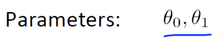
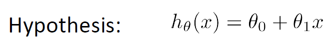
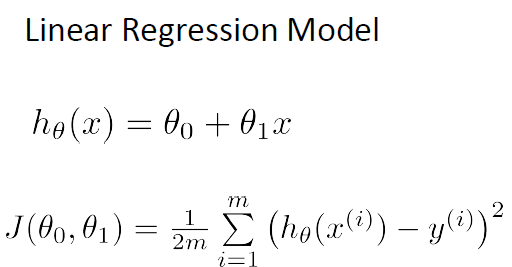
The hypothesis can be describe with this typical linear equation:
The cost function is
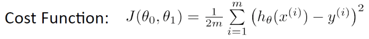
where m is the amount of data points.
Reminder again, the objective of linear regression is to minimize the cost function. Thus, the goal is to minimize J(θ0, θ1) and we will fit the linear regression parameters with data using gradient descent. There are two main function defined, derivative_J_theta() and gradient_descent() to perform gradient descent algorithm.
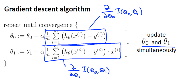
As shown in the code below, the computation mainly is using the equation express mathematically as above. The derivative_J_theta() function to compute θ0 and θ1. Next, we measure the accuracy or loss of our hypothesis function by using the cost function.
def derivative_J_theta(x, y, theta_0, theta_1):

  delta_J_theta0 = 0
  delta_J_theta1 = 0

  for i in range(len(x)):
    delta_J_theta0 +=  (((theta_1 * x[i]) + theta_0) - y[i])
    delta_J_theta1 +=  (1/x.shape[0]) * (((theta_1 * x[i]) + theta_0) - y[i]) * x[i]

  temp0 = theta_0 - (learning_rate * ((1/x.shape[0]) * delta_J_theta0) )
  temp1 = theta_1 - (learning_rate * ((1/x.shape[0]) * delta_J_theta1) )

  return temp0, temp1
def gradient_descent(x, y, learning_rate, starting_theta_0, starting_theta_1, iteration_num):
  store_theta_0 = np.empty([iteration_num])
  store_theta_1 = np.empty([iteration_num])
  # store_j_theta = []

  theta_0 = starting_theta_0
  theta_1 = starting_theta_1

  for i in range(iteration_num):
    theta_0, theta_1 = derivative_J_theta(x, y, theta_0, theta_1)
    store_theta_0[i] = theta_0
    store_theta_1[i] = theta_1
    store_j_theta = ((1/2*X.shape[0]) * ( ((theta_1 * X) + theta_0) - Y)**2)
    # store_j_theta.append((1/2*X.shape[0]) * ( ((theta_1 * X) + theta_0) - Y)**2)


  return theta_0, theta_1, store_theta_0, store_theta_1, store_j_theta
We can now training the model with small iteration number first and observe the result.
x = X
y= Y
learning_rate = 0.01
iteration_num = 10
starting_theta_0 = 0
starting_theta_1 = 0
theta_0, theta_1, store_theta_0, store_theta_1, store_j_theta = gradient_descent(x, y, learning_rate, starting_theta_0, starting_theta_1, iteration_num)
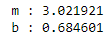
print("m : %f" %theta_0[0])
print("b : %f" %theta_1[0])
The m and b value we will obtain is 3.0219 and 0.6846 respectively.
Let’s plot the line to see how well the hypothesis fit into our data.
plt.scatter(X[:,0],Y[:,0])
plt.plot(X,(theta_1 * X) + theta_0, c='green')
plt.plot(X, X.dot(ne_theta), c='red')
plt.title('r=%f'%ne_theta[0,0])
plt.show()
The green line indicates our prediction, while red line is the normal equation.
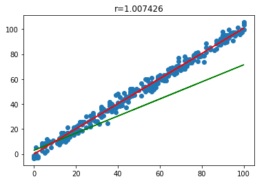
Almost there! It seem like more iteration will generate better results. We will increase the iteration number to 100.
iteration_num = 100
The m value now is 3.3572 and b is 0.9560. Plot the graph again.
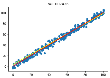
Great! The new trained parameter θ0 and θ1 are both optimized and almost align with the best fit red line. It indicated our gradient descent algorithm is working well.
From this example, we can understand clearly on the mathematics fundamental behind the univariate linear regression algorithm, and it can be very useful to perform prediction in machine learning applications.
Additional information about the differences between Gradient Descent and Normal Equation are summarized in the short notes.
Welcome to discuss more about this simple yet useful analysis technique.
Thank you for your valuable time to read this article.
This is the related repository.


Univariate Linear Regression with mathematics in Python was originally published in Becoming Human: Artificial Intelligence Magazine on Medium, where people are continuing the conversation by highlighting and responding to this story.
Voice acting is an integral component of modern video games, effectively providing much realism and immersiveness. This comes at a cost, however, as tinkerers (modders) don’t have access to the original professional voice actors used in the games’ creation processes. This usually means user generated content suffers from a lack of voiced characters, or often sub-par quality of voice recordings where recording equipment is not very good.
This is a companion post for the v1.0 release of xVASynth, a tool I’ve been working on since 2018, which aims to tackle this problem using established neural speech synthesis techniques. I’ll go into more technical detail here regarding the development process and the models used. Watch this quick intro video to see preview/summary of the app, narrated by some of the trained voices:
The main goal of this app is to provide content creators with a way to generate new voice acted lines for their projects. As such, audio quality is the top priority. A secondary objective is to provide a way to exert artistic control over the generated audio.
The models are built around datasets like LJSpeech, which is formatted as a folder full of .wav files, and an accompanying metadata.csv file containing lines for each .wav file, as follows:
<filename>|<text transcript>
Extracting audio/transcript data from games was quite easy, thanks to the very open and moddable nature of Bethesda games, and great tools like BAE, LazyAudio, and Bethesda’s Creation Kit. To start preparing the data for training, the audio files were first extracted from the game file, then decomposed into .lip and .wav files. The transcript was extracted using the Creation Kit. Following this, it was just a matter of matching up the audio files to the transcript, which was easy to do via a python script. To finalize the transcripts, a number of filtering passes were run, to exclude invalid data such as screams, shouts, music, and lines with extra unspoken text.
For the actual audio files, a couple additional pre-processing steps were required, starting with down-sampling the audio to 22050Hz mono audio. Using pydub, the audio silence was trimmed from either end, and the middle of the audio where long pauses were present (sox can also do this, but it introduced audio artifacts).
I started early experiments during this project in 2018, using Tacotron. At this point, the project was a proof of concept, and was riddled with issues, as can be seen in this video I made showcasing progress at a v0.1 pre-release version.
Though it somewhat worked, the audio quality was terrible (with very high reverb), and the output was quite unstable. The model was also very slow to load. Additionally, the model required very large datasets which limited me to voices from voice actors who also recorded audio books (The data pre-processing for which was a whole other messy can of worms). Finally, any artistic control was limited to clever use of punctuation.
Fast-forward to 2020 and the PyTorch FastPitch model by NVIDIA was released. There are several key features of this model that are useful for this project.
One of the main selling points of this model is its focus on letter-by-letter values for pitch and duration. This meant that by hijacking intermediate model values, a user would be able to have artistic control over how the audio is generated – a great plus for the acting part of voice acting.

Another plus is the support for multiple speakers per model. The best quality was still achieved when training a single speaker at a time. However, this has meant that training (or at least pre-training) voices with only a small amount of data was now possible, by grouping them up.
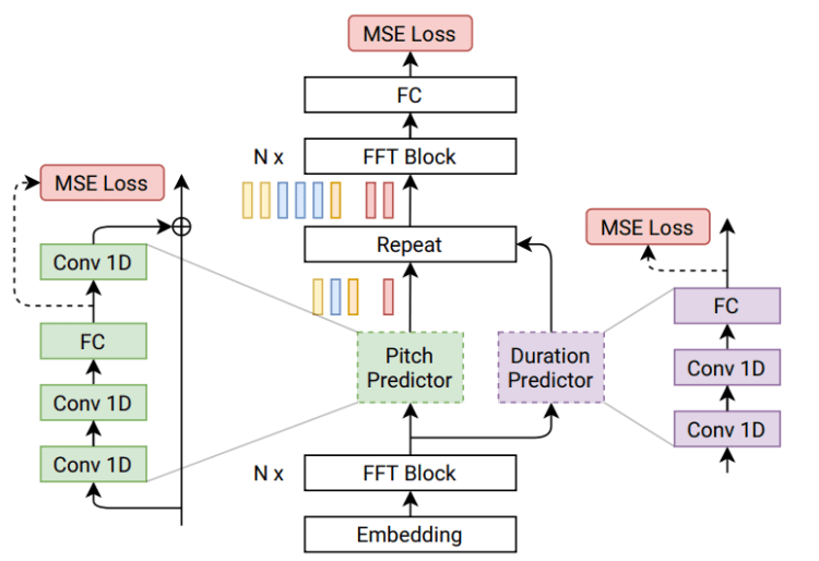
However, the most important point for this project is that audio generation was backed by a pre-trained Tacotron 2 model, instead of learning from scratch. As a pre-processing step, the Tacotron 2 model outputs mel spectrograms, and character durations which is what is used to compute the loss, as shown in the diagram above, from the paper (the pitch information is extracted using a different method).
Just like Tacotron and Tacotron 2, the FastPitch model generates mel spectrograms, so another model is needed to generate actual .wav audio files from these spectrograms. The FastPitch repo uses WaveGlow for this, which works really well.
This dependency on Tacotron 2 has meant the training has been far more quick, simple and successful. However, an issue still persists when the speaker style is very different from the one the pre-trained Tacotron 2 was trained on, LJSpeech. LJSpeech is a female speaker dataset, meaning deep male voices cannot very well be converted to the data required by FastPitch.
At the time of writing, v1.0 xVASynth comes with 34 models trained for 53 voice sets across 6 games, with many more planned for future releases. The issue with Tacotron 2 persists for most male voices, as I don’t currently have the hardware requirements to train/fine-tune a Tacotron 2 model well enough, though this is the next step after my next hardware upgrade.
The video at the top of this post details usage examples for the app, which can be downloaded from either GitHub or the Nexus.
I additionally added HiFi-GAN as an alternative vocoder to WaveGlow, which is orders of magnitude faster on the CPU, albeit at lower audio quality.
I decided to also get the ball rolling and make an example mod using this tool. People who have played Oblivion may have been haunted by the very infamous “Stop right there criminal scum” lines uttered by the seemingly psychic guards. Well, with xVASynth the nightmare can continue, in Skyrim!
Until I next upgrade hardware, the plan is to go through the very lengthy list of remaining voices for the Bethesda games currently supported (and soon to be released), with a larger focus on the female voices.
Once I can fine-tune Tacotron 2, I’ll go back through the list, then I’ll have a go at doing the really difficult voices, such as robots, ghouls, and other creatures, to see how far this can be pushed.
You can track development progress on the GitHub project page, or one of the nexus pages, where the app and models can be downloaded. There is also a discord channel set up for discussions around this you can join: https://discord.gg/nv7c6E2TzV
Generating neural speech synthesis voice acting using xVASynth was originally published in Becoming Human: Artificial Intelligence Magazine on Medium, where people are continuing the conversation by highlighting and responding to this story.
Originally from KDnuggets https://ift.tt/3i3hNnt
Originally from KDnuggets https://ift.tt/39nxfXI
According to Andrew Ng’s Machine Learning Yearning book, there are several things that might affect the variance (a.k.a. overfitting rate, or the difference between training and testing accuracy) of a model. Two of which are listed below.
Today, in this article I would like to make a proof of these theories.
Let’s now talk about the first thing first — the number of training data. Theoretically, more training samples is able to address overfitting problem pretty significantly. According to my experience of creating a CNN model for pneumonia detection (here’s the dataset), implementing ImageDataGenerator() object from Keras as an approach to augment image data did help me to reduce overall model variance. The process of data augmentation itself is done by creating random rotation, shift, zoom, etc. based on the existing train images. Essentially, the CNN model didn’t even know that those pictures are actually taken from the exact same distribution. This kind of technique is able to make as if the model being trained on large number of data. Therefore (back to the main topic), if you want to make your model to be overfitting, just use small amount of training data and never use data augmentation technique.
Time for the proof. So, the neural network architecture I displayed below is the one that I used to classify whether a person is healthy, suffers bacterial pneumonia, or suffers viral pneumonia based on their chest x-ray images.
Model: "functional_1"
_________________________________________________________________
Layer (type)                 Output Shape              Param #
=================================================================
input_1 (InputLayer)         [(None, 200, 200, 1)]     0
_________________________________________________________________
conv2d (Conv2D)              (None, 200, 200, 16)      160
_________________________________________________________________
conv2d_1 (Conv2D)            (None, 200, 200, 32)      4640
_________________________________________________________________
max_pooling2d (MaxPooling2D) (None, 100, 100, 32)      0
_________________________________________________________________
conv2d_2 (Conv2D)            (None, 100, 100, 16)      2064
_________________________________________________________________
conv2d_3 (Conv2D)            (None, 100, 100, 32)      2080
_________________________________________________________________
max_pooling2d_1 (MaxPooling2 (None, 50, 50, 32)        0
_________________________________________________________________
flatten (Flatten)            (None, 80000)             0
_________________________________________________________________
dense (Dense)                (None, 100)               8000100
_________________________________________________________________
dense_1 (Dense)              (None, 50)                5050
_________________________________________________________________
dense_2 (Dense)              (None, 3)                 153
=================================================================
Total params: 8,014,247
Trainable params: 8,014,247
Non-trainable params: 0
_________________________________________________________________
The idea behind this experiment is that, I trained the exact same model first by using image data augmentation method, and second without data augmentation. Below is how the training process looks like after 45 epochs.
Epoch 43/45
163/163 [==============================] - 17s 104ms/step - loss: 0.4973 - acc: 0.7910 - val_loss: 0.7446 - val_acc: 0.7869
Epoch 44/45
163/163 [==============================] - 17s 104ms/step - loss: 0.5017 - acc: 0.7899 - val_loss: 0.8871 - val_acc: 0.7340
Epoch 45/45
163/163 [==============================] - 17s 102ms/step - loss: 0.5007 - acc: 0.7841 - val_loss: 0.6466 - val_acc: 0.8141
As you can see the progress bar above, it’s clearly seen that the accuracy towards train and validation data seems pretty close to each other. Therefore we can just conclude that this model does not suffer overfitting.
But now let’s do the second one. I do not use data augmentation technique this time around, and below is the last 3 training epochs.
Epoch 43/45
163/163 [==============================] - 4s 26ms/step - loss: 0.0053 - acc: 0.9977 - val_loss: 5.4777 - val_acc: 0.6362
Epoch 44/45
163/163 [==============================] - 4s 26ms/step - loss: 0.0015 - acc: 0.9996 - val_loss: 5.2033 - val_acc: 0.6442
Epoch 45/45
163/163 [==============================] - 4s 27ms/step - loss: 2.3021e-04 - acc: 1.0000 - val_loss: 5.8940 - val_acc: 0.6410
Alright, so the result above shows that the model is extremely overfitting that the training accuracy touches exactly 100% while at the same time the validation accuracy does not even reach 65%. So ya, back to the topic again. IF YOU WANNA MAKE YOUR MODEL OVERFIT THEN JUST USE SMALL AMOUNT OF DATA. Keep that in mind.
Next up, let’s talk about how the number of features affect classification performance. Different to the previous one, here I am going to use potato leaf disease dataset (it’s here). What basically I wanna perform here is to train two CNN models (again), where the first one is using max-pooling while the next one doesn’t. So below is how the first model looks like.
Model: "sequential_6"
_________________________________________________________________
Layer (type)                 Output Shape              Param #
=================================================================
conv2d_10 (Conv2D)           (None, 254, 254, 16)      448
_________________________________________________________________
conv2d_11 (Conv2D)           (None, 252, 252, 32)      4640
_________________________________________________________________
max_pooling2d_1 (MaxPooling2 (None, 63, 63, 32)        0
_________________________________________________________________
flatten_6 (Flatten)          (None, 127008)            0
_________________________________________________________________
dense_18 (Dense)             (None, 100)               12700900
_________________________________________________________________
dense_19 (Dense)             (None, 50)                5050
_________________________________________________________________
dense_20 (Dense)             (None, 3)                 153
=================================================================
Total params: 12,711,191
Trainable params: 12,711,191
Non-trainable params: 0
_________________________________________________________________
As you can see the model summary above, the max-pooling layer is placed right after the last convolution layer. — Well, the size of this pooling layer is 4×4, but it’s just not mentioned in this summary. Also, note that the number of neurons in the flatten layer is only 127,008.
The output showing the training progress bar looks like below. Here you can see that the model is performing excellent since the accuracy towards validation data is reaching up to 93%.
Epoch 18/20
23/23 [==============================] - 1s 31ms/step - loss: 1.0573e-05 - acc: 1.0000 - val_loss: 0.3191 - val_acc: 0.9389
Epoch 19/20
23/23 [==============================] - 1s 31ms/step - loss: 9.6892e-06 - acc: 1.0000 - val_loss: 0.3215 - val_acc: 0.9389
Epoch 20/20
23/23 [==============================] - 1s 31ms/step - loss: 8.9155e-06 - acc: 1.0000 - val_loss: 0.3233 - val_acc: 0.9389
But remember that we want the model to be AS OVERFIT AS POSSIBLE. So my approach here is to modify the CNN such that it no longer contains max-pooling layer. Below is the detail of the modified CNN model.
Model: "sequential_4"
_________________________________________________________________
Layer (type)                 Output Shape              Param #
=================================================================
conv2d_6 (Conv2D)            (None, 254, 254, 16)      448
_________________________________________________________________
conv2d_7 (Conv2D)            (None, 252, 252, 32)      4640
_________________________________________________________________
flatten_4 (Flatten)          (None, 2032128)           0
_________________________________________________________________
dense_12 (Dense)             (None, 100)               203212900
_________________________________________________________________
dense_13 (Dense)             (None, 50)                5050
_________________________________________________________________
dense_14 (Dense)             (None, 3)                 153
=================================================================
Total params: 203,223,191
Trainable params: 203,223,191
Non-trainable params: 0
_________________________________________________________________
Now, you can see the summary above that the number of neurons in the flatten layer is 2,032,128. This number is a lot more compared to the one that we see in the CNN which contains pooling layer in it. Remember, in CNN the actual classification task is done by the dense layer, which basically means that the number of neurons in this flatten layer acts kinda like the number of the input features.
Theoretically speaking, the absence of the pooling layer will cause the model to get more overfit due to the fact that the number of features is a lot higher compared to the previous CNN model. In order to prove, let’s just fit the model and see the result below.
Epoch 15/20
23/23 [==============================] - 2s 65ms/step - loss: 0.0016 - acc: 1.0000 - val_loss: 2.4898 - val_acc: 0.6667
Epoch 16/20
23/23 [==============================] - 2s 68ms/step - loss: 0.0014 - acc: 1.0000 - val_loss: 2.5055 - val_acc: 0.6667
Epoch 17/20
23/23 [==============================] - 2s 66ms/step - loss: 0.0013 - acc: 1.0000 - val_loss: 2.5193 - val_acc: 0.6667
Epoch 18/20
23/23 [==============================] - 1s 65ms/step - loss: 0.0011 - acc: 1.0000 - val_loss: 2.5339 - val_acc: 0.6611
Epoch 19/20
23/23 [==============================] - 2s 65ms/step - loss: 0.0010 - acc: 1.0000 - val_loss: 2.5476 - val_acc: 0.6611
Epoch 20/20
23/23 [==============================] - 2s 65ms/step - loss: 9.2123e-04 - acc: 1.0000 - val_loss: 2.5602 - val_acc: 0.6611
And yes, we’ve got to our goal. We can clearly see here that the validation accuracy is only 66% while at the same time the training accuracy is exactly 100%.
Long story short here’s two things that you can do if you wanna overfit your model:
I hope by knowing how to make a model being overfit, now you know how not to do so. Thanks for reading 🙂
How to Overfit Your Model was originally published in Becoming Human: Artificial Intelligence Magazine on Medium, where people are continuing the conversation by highlighting and responding to this story.
Via https://becominghuman.ai/how-to-overfit-your-model-e1a84906a361?source=rss—-5e5bef33608a—4
source https://365datascience.weebly.com/the-best-data-science-blog-2020/how-to-overfit-your-model

Today, emerging technologies have transformed nearly every aspect of human lives. The Healthcare industry has also been revolutionized by the emergence of healthcare software in the market. Healthcare software streamlines healthcare delivery and accelerates the process and helps healthcare providers manage and perform their work more efficiently.
The global healthcare software development market is already massive and is expected to grow even higher, with a growth of 5.8 percent to reach 19.3 billion dollars by 2025. According to the Deloitte Global Healthcare Outlook report, the global spending on healthcare software development is expected to rise by 5 percent over five years 2019–2023. No surprise, healthcare software development demands are continually increasing. Moreover, the pandemic covid-19 has disrupted the entire healthcare industry and has given an explosive rise in healthcare software demands.
The software industry offers numerous services to the healthcare industry. The benefits that the healthcare industry can get from software development are listed below:
Benefits through novel technologies
Benefits for Doctors
Benefits for Patients
Benefits for Healthcare Organizations
The Healthcare industry is continually growing, and with this growth, the demands for software development is also increasing. Software development companies are continuously working to improve and bring innovation to this industry. The Healthcare industry is among those which depend on high efficiency and accuracy. The emerging technologies, including AI, IoT and Blockchain, possess the capability to deliver required software solutions.
What are the benefits of Healthcare Software Development? was originally published in Becoming Human: Artificial Intelligence Magazine on Medium, where people are continuing the conversation by highlighting and responding to this story.
