365 Data Science is an online educational career website that offers the incredible opportunity to find your way into the data science world no matter your previous knowledge and experience.
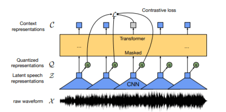
The raw speech is passed through a feature encoder (temporal CNN blocks + layer norm + GeLU activation) and the latent features are extracted.
The latent features are continuous and we need to discretize them for learning speech representations so these features are quantized using some code books to obtain the quantized features.
The quantized features are masked with some (arbitrary) probability. We don’t mask the inputs to the quantization module, instead we mask the output of quantized module in the latent feature encoder space. With some arbitrary probability we select the indices and mask them along with M-consecutive indices w.r.t sampled indices.
These features are passed through a contextualized model like transformers and the masked features are predicted.
Machine Learning Jobs
Problems with Quantization:
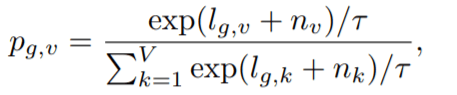
We choose quantized vector representations each from multiple codebooks and then they are concatenated. But how to choose the quantized vector? We choose the one which is having minimum difference with the extracted feature and this operation is done using argmin operator which is converted into argmax by introducing negation. But argmax is non-differentiable hence backprop is a problem. So here comes the role of Gumbel SoftMax which provides a way of choosing a quantized vector representation from codebooks, with the benefits of being differentiable in nature. So, we use argmax in forward prop and while backprop we use Gumbel SoftMax.
Gumbel SoftMax
T= non-negative temperature constant ;nv, nk= Gumbel Noise ; here, the terml(g,v)represents code at indexvfrom codebook id = g
We try to predict the quantized vectors from the set of distractors (distractors are uniformly sampled from other masked time steps from the same utterance) at the time steps which are masked by minimizing the loss between prediction and the quantized vector at that certain masked time steps.
What are the losses to be minimized?
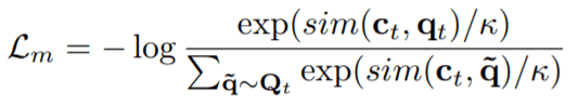
Contrastive Loss (Lm): The objective of this loss is to bring the prediction of current masked timestep closer to the actual quantized latent speech representation which should have been there at the same time step, followed by pushing the prediction far away from distractors.
Here,sim()function is cosine-similarity function and the termCtis output of the model at timestep=t.
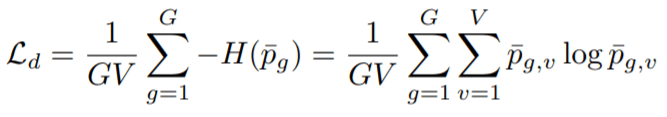
Diversity Loss (Ld): This loss objective is responsible for bringing in equal opportunities of selection for all the V entries present in each of the G-codebooks. So, we maximize the entropy of averaged SoftMax distribution for each of the entries in the codebook and to bring in equal opportunity across a batch of utterances. This is naïve SoftMax which doesn’t include non-negative temperature coefficient and Gumbel noise.
Here, probability term represents probability of finding v-th entry from g-th codebook.
Total Loss:
Often, the setting is little bit changed when we pretrain on smaller Librispeech dataset, by introducing L2 penalty in the activations of the final layer of feature encoder to regularize training and reducing the gradient by a factor of 10. The authors have also suggested to remove the layer normalization step in the feature encoder and normalizing the output of only first layer of feature encoder. Checkpoint is set for the epoch where contrastive loss is minimum on the validation set.
For decoding, there are two schools of thoughts, one is via a 4-gram LM and other idea is to use a pretrained (on Librispeech LM corpus) Transformer LM, followed by choosing the best of both worlds using beam search decoding scheme. For more details I would request you to see these details in the original paper.
Fine-tuning:
The pretrained model can be finetuned for downstream tasks like Speech Recognition using little amount of labelled dataset. What we need to do is to just apply a linear projection layer over transformer decoder to convert the dimension size equal to the vocabulary size of the data on which you are training and minimizing the CTC loss objective.
Results:
The authors have developed Phoneme Recognizer for TIMIT dataset and have achieved SOTA, following standard protocol of collapsing the phone labels into 39 labelled classes. The results show that jointly learning discrete speech units with contextualized representations achieves substantially better results than fixed units learned in older architectures. The authors have demonstrated the feasibility of ultra-low resource speech recognition: when using only 10 minutes of labelled data, they achieved word error rate (WER) 4.8/8.2 on the clean/other test sets of Librispeech. The authors have set a new state of the art on TIMIT phoneme recognition as well as the 100-hour clean subset of Librispeech. Moreover, when lowering the amount of labelled data to just one hour, this approach still outperforms the previous state of the art self-training method while using 100 times less labelled data and the same amount of unlabelled data. When all 960 hours of labelled data were used from Librispeech, then the model achieved 1.8/3.3 WER
I have explained the mechanism of the architecture and the observations but if you are interested about the exact figures in the results obtained and the dataset used for training and testing, I will suggest to refer to this paper. It will help you gain more insights and the original paper will look easier to understand once you finish this article. I have tried to explain it lucidly from my end, hoping that it might have helped you and I thank you for your patience. Hoping the best for you in your journey, thankyou until next time!
If you are considering starting a career path in machine learning and data science, then there is a great deal to learn theoretically, along with gaining practical skills in applying a broad range of techniques. This comprehensive learning plan will guide you to start on this path, and it is all available for free.
Model monitoring using a model metric stack is essential to put a feedback loop from a deployed ML model back to model building so that ML models can constantly improve itself under different scenarios.
The first issue in 2021 brings you a great blog about Monte Carlo Integration – in Python; An overview of main Machine Learning algorithms you need to know in 2021; SQL vs NoSQL: 7 Key Takeaways; Generating Beautiful Neural Network Visualizations – how to; MuZero – may be the most important Machine Learning system ever created; and much more!
Marketing data science – data science related to marketing – is now a significant part of marketing. Some of it directly competes with traditional marketing research and many marketing researchers may wonder what the future holds in store for it.
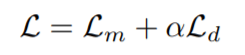
In computer vision world, objects can be viewed through images. And classifying, tagging, segmenting and annotating these are images are important to make the objects of interest perceivable to machines. And in AI world, computer vision is playing big role helping the models understand the scenario around the world making AI possible through machine learning or deep learning.
What is Image Segmentation?
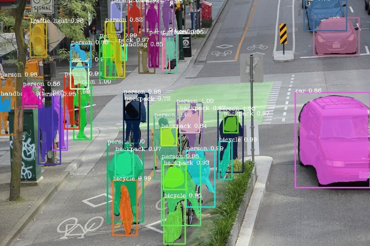
Image segmentation is the process of partitioning of digital images into various parts or regions (of pixels) reducing the complexities of understanding the images to machines. Image segmentation could also involve separating the foreground from the background or assembling of pixels based on various similarities in the color or shape.
Image Segmentation in Machine Learning
Various image segmentation algorithms are used to split and group a certain set of pixels together from the image. It is actually the task of assigning the labels to pixels and the pixels with the same label fall under a category where they have some or the other thing common in them.
Artificial Intelligence Jobs
And using these labels, you can specify boundaries, draw lines, and separate the most required objects in an image from the rest of the unimportant one.
In machine learning — image segmentation helps to make these identified labels further use for supervised and unsupervised training that is mainly required to develop machine learning based AI model. Image segmentation is used for image processing into various types of computer vision projects.
Why Image Segmentation is needed?
In image recognition system, segmentation is an important stage that helps to extract the object of interest from an image which is further used for processing like recognition and description. Image segmentation is the practice for classifying the image pixels.
And there are various image segmentation techniques are sued to segment the images depending on the types of images. Actually, compared to segmentation of color images is more complicated compare to monochrome images.
Basically, there are two broader categories of segmentation techniques — Edge-Based & Region-based, but various other image segmentation techniques are required to develop various AI models.
Threshold Method
Edge Based Segmentation
Region Based Segmentation
Clustering Based Segmentation
Watershed Based Method
Partial Differential Equation Based Segmentation Method
Artificial Neural Network Based Segmentation
All these types of image segmentation techniques are used for object recognition and detection in various types of AI model applications. In satellite imagery, image segmentation can be used to detect roads, bridges while in medical imaging analysis, it can be used to detect cancer. In image annotation, semantic segmentation is used to make the objects in the single class recognizable to machines.
The need for image segmentation is very much important especially in the AI world. Image segmentation applications are becoming more important due to demand in AI industry that is dedicatedly involved in developing the machine and deep leering models for different fields.
Anolytics is one of the top companies providing the data annotation service with expertise in image annotation to create the high-quality training data for machine learning models developed through computer vision algorithms. It is also offering the semantic image segmentation with high-level of precision for varied fields healthcare, retail, automotive, agriculture and autonomous vehicles.
Docking Proteins to Deny Disease: Computational Considerations for Simulating Protein-Ligand Interaction
Molecular Docking for Drug Discovery
Molecular docking is a powerful tool for studying biological macromolecules and their binding partners. This amounts to a complex and varied field of study, but of particular interest to the drug discovery industry is the computational study of interactions between physiologically important proteins and small molecules.
This is an effective way to search for small molecule drug candidates that bind to a native human protein, either attenuating or enhancing activity to ameliorate some disease condition. Or, it could mean binding to and blocking a protein used by pathogens like viruses or bacteria to hijack human cells.
Protein-ligand interaction in health and disease.Left:5-HT3 receptor with serotonin molecules bound, an interaction that plays important roles in the central nervous systems.Right:Mpro, a major protease of the SARS-CoV-2 coronavirus responsible for COVID-19, bound to the inhibitorBoceprevir.
Drug discovery has come a long way from its inception. The first drugs used to treat maladies were probably discovered in prehistory in the same way as the first recreational drugs were: someone noticing strange effects after ingesting plant or animal matter out of boredom, hunger, or curiosity. This knowledge would have spread rapidly by word of mouth and observation. Even orangutans have been observed producing and using medicine by chewing leaves into a foamy lather to use as a topical painkiller. The practice is local to orangutans in only a few places in Borneo, so it was almost certainly discovered and passed on rather than as a result of instinctual use, which is actually quite common even among invertebrates.
Artificial Intelligence Jobs
Historical drug discovery from the times of ancient Sumerians to the Renaissance in Europe was also a matter of observation and guesswork. This persisted as the main method for drug discovery well into the 20th century. Many of the most impactful modern medicines were discovered by observation and happenstance, including vaccines, discovered by Edward Jenner in the 1700s after observing dairy maids that were immune to smallpox thanks to exposure to the bovine version of the disease, and antibiotics, discovered by Alexander Fleming as a side-effect of keeping a somewhat messy lab.
Isolating Large Libraries of Chemical Compounds
Discovery by observation provides hints at where to look, and researchers and a burgeoning pharmacology industry began to systematically isolate compounds from nature to screen them for drug activity, especially after World War II. But it’s easier to isolate (and later synthesize) large libraries of chemical compounds than it is to test each one in a cell culture or animal model for every possible disease. This has culminated in many pharmaceutical companies maintaining vast libraries of small molecule compounds with likely physiological activity. As a result, choosing which compounds out of thousands are worth studying more closely to combat a given disease, known as lead generation, is the first hurdle to leap in the modern drug discovery process. Automated high-throughput screening is a promising tool for discovering leads, at least when it’s done intelligently. Computational chemistry, on the other hand, has the potential to be vastly more efficient than any sort of screening you can do in a wet lab.
There are two main categories docking simulations can fall under: static/rigid, versus flexible/soft.
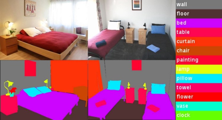
Conceptually these are related to two mental models of how proteins interact with other molecules, including other proteins: the lock and key model and the induced fit model. The latter is sometimes referred to as the “glove” model, relating to the way that a latex glove stretches to accommodate and take the shape of a hand. These aren’t so much competing models as they are different levels of abstraction. Proteins are almost never going to be perfectly rigid under physiological temperatures and concentrations.
From our computational perspective, flexible docking is closer to actual conditions experienced by proteins and ligands, but rigid docking will clearly be much faster to compute. A useful compromise between speed and precision is to screen against several different static structural conformations of the same protein. That being said, it’s hard to get all of the details right in a more complex simulation such as flexible docking, and in those cases it’s better to be less precise but more accurate.
Models of protein-ligand interaction, lock-and-key interaction and induced fit, or “glove” binding. These ideas about protein binding are parallelled in rigid and flexible docking simulation, respectively.
Protein-ligand docking as a means for lead generation has many parallels to deep learning. The technique has taken on a qualitatively different character over the last few decades, thanks to Moore’s law and related drivers of readily available computational power.
Although it’s widely accepted that Moore’s law isn’t really active anymore, at least in terms of the number of transistors that can be packed onto a given piece of silicon, the development of parallel computing in hardware accelerators like general-purpose graphics processing units (GP-GPUs), field programmable gate arrays (FPGAs), and application specific integrated circuits (ASICs) has ensured that we still see impressive yearly improvements in computation per Watt or computation per dollar.
As we’ll discuss in this post, some molecular docking software programs have started to take advantage of GPU computation, and hybrid methodologies that implement molecular docking and deep learning inference side by side can speed up virtual screening by more than 2 orders of magnitude.
Even without explicit support for parallelization, modern computation has driven the adoption of protein-ligand docking for high throughput virtual screening. Docking is one of several strategies for screening that include predicting quantitative structure-activity relationship (QSAR) and virtual screening based on chemical characteristics and metrics associated with a large library.
More Compute, More Molecules
Simulated protein-ligand docking has historically been used in a more focused manner. Until recently, you’d be more likely to perform a docking study with only one or a handful of ligands. This generally entails a far amount of manual ligand processing as well as direct inspection of the protein-ligand interaction, and would be conducted at the hands of a human operator with a huge degree of technical knowledge (or as it says in the non-compete in your contract proprietary “know-how”).
These days it’s much more feasible to screen hundreds to thousands of small molecules against a handful of different conformations of the same protein, and it’s considered good practice to use a few different docking programs as well, as they all have their own idiosyncrasies. With each docking simulation typically taking on the order of seconds (for one ligand on one CPU), this can take a significant amount of time and compute even when spread out across 64 or so CPU cores. For large screens, it pays to use a program that can distribute the workload over several machines or nodes in a cluster.
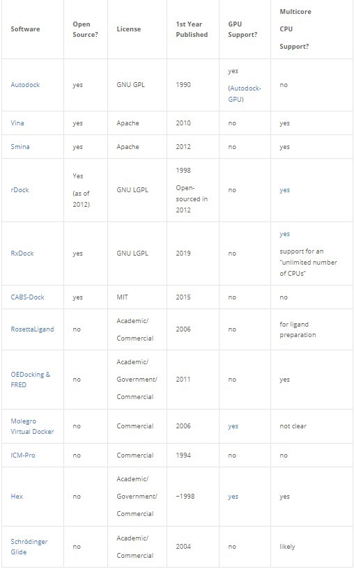
Non-exhaustive list of software for protein-ligand docking simulation.
We can see in the table above that very few docking programs have been designed or modified to take advantage of the rapid progress in GPU capabilities. In that regard molecular docking trails deep learning by 6 years or so.
Autodock-GPU (open source option), Molegro Virtual Docker, and Hex are the only examples in the table that have GPU support. Of those, Autodock-GPU is the only open source option, Hex has a free academic license, and Molegro Virtual Docker doesn’t list pricing for the license on the website. Autodock 4 has also been implemented to take advantage of FPGAs as well, so if your HPC capabilities include FPGAs they don’t have to go to waste.
Even if using a docking program that doesn’t support GPU computation, there are other ways to take advantage of hardware acceleration by combining physics-based docking simulation with deep learning, and other machine learning models.
The Fastest Docking Simulation is One That Doesn’t Run at All
Even if most molecular docking software doesn’t readily support GPU acceleration, there’s an easy and straightforward way to take advantage of GPUs and all of the technical development in GPU computing that has been spurred on by the rising value proposition of deep learning, and that’s to find a place in your workflow where you actually can plug in some deep learning.
Neural networks of even modest depth are technically capable of universal function approximation, and researchers have shown their utility in approximating many physical phenomena at various scales. Deep NNs can provide shortcuts by learning relationships between structures and molecule activity directly, but they can also work together with a molecular docking program to make high throughput screening more efficient.
Austin Clyde describes a deep learning pre-filtering technique for high throughput virtual screening using a modified 50 layer ResNet neural network. In this scheme, the neural network predicts which ligands (out of a chemical library of more than 100 million compounds) are more likely to demonstrate strong interaction with the target protein. Those chosen ligands then enter the molecular docking pipeline to be docked with AutoDock-GPU. This vastly decreases the ligand search space while still discovering the majority of the best lead candidates.
Remarkably the ResNet model is trained to predict the best docking candidates based on a 2D image of each small molecule, essentially replacing the human intuition that might go into choosing candidates for screening.
The optimal use of available compute depends on the relationship between the GPU(s) and the number of CPU cores on the machine used for screening. To fully take advantage of the GPU (running ResNet) and the CPU cores (orchestrating docking) the researchers adjust the decision threshold to screen out different proportions of the molecular library. Clyde gave examples: screening only the top 1% of molecules chosen by the ResNet retains 50% of the true top 1% and 70% of the top 0.05% of molecules, and screening the top 10% chosen by ResNet recovers all of the top 0.1%. In some cases Clyde describes a speedup of 130x over naively screening all candidates. A technical description of this project, denoted IMPECCABLE (an acronym that is surely trying too hard), is available on Arxiv.
GPU and Multicore Examples
We looked at 2 open source molecular docking programs, AutoDock-GPU and Smina.
While these are both in the AutoDock lineage (Autodock Vina succeeds AutoDock, and Smina is a fork of Vina with emphasis on custom scoring functions), they have different computational strengths. AutoDock-GPU, as you can guess, supports running its “embarrassingly parallel” Lamarckian Genetic Algorithm on the GPU, while Smina can take good advantage of multiple cpu cores up to the value assigned by the –exhaustiveness flag.
Smina uses a different algorithm, the Broyden-Fletcher-Goldfarb-Shanno (BFGS) algorithm so the comparison isn’t direct, but the run speeds are quite comparable using the default settings. Increasing the thoroughness of search by setting -nrun (used by AutoDock-GPU) and –exhaustiveness (used by Smina) flags to high values, however, favors the multicore Smina over the GPU-enabled AutoDock.
Smina is available for download as a static binary on Sourceforge, or you can download and build the source code from Github. You’ll have to make AutoDock-GPU from source if you want to follow along, following the instructions from their Github repository. You’ll need either CUDA or OpenCL installed, and make sure to pay attention to environmental variables you’ll need to parametrize the build: DEVICE, NUMWI, GPU_LIBRARY_PATH and GPU_INCLUDE_PATH.
We used PyMol, openbabel and this script to prepare the pdb structure 1gpk for molecular docking with Smina. Preparation for AutoDock-GPU was a little more involved, as it relies on building a grid with autodock4, part of AutoDockTools. Taking inspiration from this thread on bioinformatics stack exchange, and taking the .pdbqt files prepared for docking with Smina as a starting point, you can use the following commands to prepare the map and grid files for AutoDock:
cd <path_to_MGLTools>/MGLToolsPckgs/AutoDockTools/Utilities24/
# after placing your pdbqt files in the Utilities24 folder
# NB You’ll need to use the included pythonsh version of python,
That should give the files you need to run AutoDock-GPU, but it can be a pain to install all the AutoDockTools on top of building AutoDock-GPU in the first place, so feel free to download the example files here.
To run docking with Smina, cd to the directory with the Smina binary and your pdbqt files for docking, then run:
And you should get some results that look similar to:
One advantage of Smina over Vina is the convenience flags for autoboxing your ligand. This allows you to automatically define the docking search space based on a ligand structure that was removed from a known binding pocket on your protein. Vina requires you to instead define the x,y,z, center coordinates and search volume.
Smina achieved a docking runtime of just over 1 second on 1 CPU for the 1gpk structure, with the default exhaustiveness of 1. Let’s see if AutoDock-GPU can do any better:
Note that your autodock executable may have a slightly different filename if you used different parameters when building. We can see that AutoDock-GPU was slightly faster than Smina in this example, almost by a factor of 2 in fact. But if we want to run docking with more precision by expanding the search, we can ramp up the -nrun and –exhaustiveness flags for some surprising results.
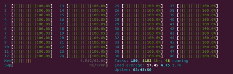
Running smina with exhaustiveness of 1000 gives us a very satisfying CPU usage that looks great when visualized with htop, and a runtime of about 20 seconds.
If we do something similar with AutoDock-GPU and the -nrun flag:
We get a runtime of just over 2 minutes. As mentioned earlier, accuracy is more important than precision when it comes to finding good drug candidates, and using 1000 for -nrun or –exhaustiveness is a truly exaggerated and preposterous way to set up your docking run (values around 8 are much more reasonable). Nonetheless, it may be more beneficial to adopt a complementary hybrid approach for high-throughput virtual screening, running docking on multiple CPU cores and using deep learning and GPUs to filter candidates, as described above for the IMPECCABLE pipeline.
In any case, speed doesn’t matter if we can’t trust the results so it pays to visually inspect docking results every once in a while.
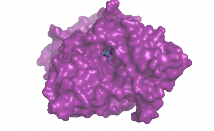
Re-docking Huperzine to acetylcholinesterase (PDB ID 1gpk). The turquoise small molecule is the output from docking program Smina. The re-docked position overlaps substantially with the true ligand position from the solved structure, in pink.
Hopefully this whirlwind tour of an article has helped to pique your interest in molecular docking. And now you can see how high throughput virtual screening can take advantage of modern multicore CPUs and GPU accelerators to blaze through vast compound libraries.
This application of compute to find chemical candidates for drugs in a targeted manner, especially when it’s done with a clever combination of machine learning and algorithmic simulation, has the potential to find new remedies faster, with fewer side-effects and better efficacy.
Unhidden Organizational Debt of Machine Learning Teams — part 1
image source: wallhere.com
The Lord Governor rose from his seat and gazed around the packed arena with pride.
“Unleash the Datum Sorcerers!” he thundered, raising his arms skywards. The spectators in their thousands roared in response.
The Warlord standing at one side of the governor turned towards him and saluted. “Are we certain, my lord?” he asked the Governor with a slight tremble in his voice.
“Indeed! The arena has been prepared! The people have gathered! The datum stones have been retrieved! Even the Emperor has granted his approval! It is time!”
Artificial Intelligence Jobs
“Very well, my lord. Just a little matter regarding the sorcerers… they, um,” the Warlord hesitated before continuing, “the last of the sorcerers died a week ago.”
“What? All of my sorcerers are dead? How can that be! We had so many of them!” the Lord Governor was aghast.
“Yes, yes. They, err, exited our world gradually, one by one, out of starvation. The Human Resource Priests had diagnosed that the sorcerers were emaciated for lack of datum.”
“Bah! I always knew one could not rely on this hocus-pocus of sorcery,” asserted the Governor, and continued, “Very well, summon the Mystic Legion Elves instead. I am sure they have learned to automate the datum gems without needing the sorcerers.”
“Very well, my lord. Just a little matter regarding the elves… they died out even before the sorcerers. They suffered from a strange unfamiliar affliction. Some of our Human Resource Priests gave it a new name — Ennui.”
The Governor stared up at the sky, with shock enveloping him. Thousands of impatient eyes from every corner of the arena were upon him. His stomach churned with the nauseating weight of their restless expectations.
“What about the Datum Alchemists? I never understood why sorcery is different from alchemy. I don’t see why the Alchemists cannot create the automaton. Can you call for the Alchemists, or are they all dead too?” the Governed glared at the Warlord.
“Very well, my lord. Just the little matter…” the Warlord faltered.
“Is EVERYONE dead?!” the Governor screamed, “Who remains among my Automaton Inquisition Troops?”
“There is, uh, one Datum Sorcery Manager, one Principal Lord of the Elves, and one Datum Alchemy Director.”
As the Governor sank back into his throne in resignation, he could hear the distant sounds of the Emperor’s army marching towards the arena…
You might have read the paper Hidden Technical Debt in Machine Learning Systems (Neurips 2015). If not, I highly recommend it. It is an excellent discussion of the technical risks and challenges associated with building and maintaining machine learning (ML) systems. Recently, going back to this article led me to ponder about an orthogonal set of challenges hindering the efforts to build, maintain, iterate and improve ML products — organizing the ML practitioners in a company. Instead of continuing to ponder in private, I felt a series of posts (starting with this one) can help me, and possibly others, unravel these organizational aspects. For the sake of a fancy sounding title, let’s call this series — “Unhidden Organizational Debt of Machine Learning Teams”.
Organizational debt isn’t a new concept. I am sure it is as old as organizations themselves. Organizational debt can, and does, accumulate in any type of company. Several articles and probably books have been written about it. It’s time to start tackling organizational debt is an example of one such recent article, which also links to several other articles (I chose to cite this article because it too is in the form of a LinkedIn post with no peer review — very much like this one!). Tech companies are not immune to organizational debt, be they a funding-starved startup or an aging behemoth. Despite their penchant for regular restructuring, the dynamic nature of the tech industry means that their organizational structure of these companies is always playing catch up with the changing day-to-day reality.
In this series of articles, however, you and I are going to zoom in to look at organizational debt specifically in terms of the people behind the development of ML systems and products. To further narrow down our scope, we will only think in terms of medium sized organizations that either have a significant software branch, or are a full-fledged software company (that leaves out startups which don’t have rigid org structures and very large companies which can be considered as conglomerates of multiple smaller ones).
Tackling these issues in the form of Why, Who, Where, What, When, and How seemed like an interesting design choice to me. This post will focus on the Why and the Who.
Why does ML organizational debt accumulate?
Since machine learning is a relatively new frontier for most tech organizations, they have only recently started forming their ML teams, often from scratch. Organizational leaders such as VPs or executives may not have a lot of prior experience of building and managing ML teams. For many of them, it might be the first time that they have a ML team in their department or organization.
While at a high level, ML development appears deceptively similar to traditional software development, anyone using ML in the industry will tell you that it differs significantly in most aspects ranging from ideation to deployment. However, with a lack of ML experience at the leadership level, there can be a gap in the understanding of the nuances of ML development and unreasonable expectations of quick turnarounds or ‘magical’ solutions. The ML teams and team leaders may then resort to quick and dirty solutions leading to a pile up of mainly technical, but also organizational debt (of course, this is also applicable to software at large, but lack of awareness and the inherent uncertainty can make it harder with respect to ML).
Coming back to the organizational aspects, as a company slowly increases its investment in data and ML, the evolution of the ML team(s) often tends to be ad-hoc, reactive and ill-designed. The skills and responsibilities of the ML teams turn out to be varied or inconsistent, and often misunderstood. All this leads to gradual accumulation of organizational debt.
On top of all this, there are no well-established best practices on organizing or managing ML teams. In fact, even the skills and tasks associated with the same job title vary significantly across companies. To underscore this, and to ensure that we are all on the same page for the remainder of the discussion, let us look at the common job titles, their multiple interpretations and the underlying skillsets. This brings us to the Who!
The Who’s-who of Machine Learning
DS aka Data Scientist (aka Datum Sorcerer): As DS became the most sought-after magical ability a few years ago with both job-seekers and job-givers coveting it, it led to a diversification of what DS implies. However, I think the responsibilities have coalesced into a few major categories. When a company thinks of a “data scientist” creature, it may be imagining any of the below:
DS-?: responsible for understanding a business problem and building data-driven solutions that will go into production, i.e., typically training ML models, including the processes of data munging, dataset creation, and so on. Sometimes also referred to as Machine Learning Scientist, Research Scientist, and other prefixes ( *-Scientist).
DS-?: responsible for munging, mining and analysing data, gathering insights, and answering business questions with data, i.e., product analytics, behavior analytics, A/B testing design & analysis, causal relationships, etc. Often called as Data Analyst, or the fancier, Decision Scientist.
DS-ƛ: responsible for both building/training ML models and deploying them into production, i.e., model serving which includes constructing the data ingestion pipelines, postprocessing and delivery of predictions, MLOps, etc. Sometimes also referred to as Applied Scientist, Full-stack Data Scientist, and more commonly, Machine Learning Engineer.
MLE aka Machine Learning Engineer (aka Mystic Legion Elf): Some time after DS had blasted onto the scene, a new creature started making an appearance. It was named MLE. In the initial days while MLE might have meant bringing the engineering chops to be able to utilize the data science models, it ended up getting morphed into two major species:
MLE-?: responsible for taking trained ML models and deploying them into production environments, i.e., model serving which includes MLOps, constructing the data ingestion pipelines, postprocessing and delivery of predictions. Sometimes, they go by an even more mouthful of a title- Software Engineer, Machine Learning.
MLE-ƛ: responsible not just for productionizing ML models, but also for training them in the first place by understanding the business, the problems and the data. As evident from above, sometimes also called as Applied Scientist, Full-stack Data Scientist, or plain old, Data Scientist.
DA aka Data Analyst (aka Datum Alchemist): These are some of the ancient creatures who have traversed both tech and non-tech companies since time immemorial. They also took on different names with different permutations of the spell-binding words like business, data, intelligence, analysis, analytics, research, etc. In the context of tech-ish companies with a focus on data science and/or machine learning, they may frequently be grouped into two varieties:
DA-?: responsible for munging and analysing data and generating insights, i.e., product analytics, behavior analytics, A/B testing design & analysis, causal relationships, etc. If this sounds familiar, it is because they sometimes go by the supposedly fancier title- Data Scientist.
DA-??: responsible mainly for data analysis and gathering insights, however, on the rare occasion, resorts to training ML models to generate predictions. Often seen in companies that are beginning to test the potions of machine learning. They are likely to eventually transform their title to Data Scientist.
SWE-ML aka Software Engineer, Machine Learning (aka regular Elf with a dose of mysticism): While the two halves of the name are essential components to this whole discussion, their combination as a title is a relatively new phenomenon. Of course, previous decades had many pioneering creatures who just went by the title of Software Engineer but who not just used ML, but laid the foundation for the emergence of the field of Data Science and Machine Learning. In a sense, they were the progenitors of several of the above species. In current times, however, creatures adopting this name are mainly of the below varieties:
SWE-ML-?: responsible for taking trained ML models and deploying them into production environments, i.e., model serving which includes the MLOps, constructing the data ingestion pipelines, postprocessing and delivery of predictions. Sometimes go by the shorter title, Machine Learning Engineer.
SWE-ML-ε: responsible for software engineering and working alongside MLEs or DSs in the ML teams. Has enough understanding of ML to steer clear of it but occasionally helps out with some MLOps. Usually go by the adornment-free title, Software Engineer.
DE aka Data Engineer (aka Datum Extractor): This is among the oldest and the least ambiguous of the creatures (perhaps due to the marked history). However, one does occasionally come across a couple of variants:
DE-?: responsible for extracting, receiving, processing, transforming, curating, storing, supplying and accessorizing data. In other words, if they don’t supply the datum gems, all the sorcerers, alchemists, and mystic elves will be nothing but idle and bored creatures.
DE-??: responsible for all the data engineering, but also have to step in to productionize ML models by building the data pipelines and other surrounding infrastructure to model serving. May eventually refashion their title to Machine Learning Engineer.
As we see, the same title implies different skills and responsibilities in different organizations. No matter what variants and combinations of titles are present in a single organization, it is critical that, for magic to happen, all the necessary skills are covered sufficiently:
? = building ML models
? = productionizing ML models
? = data analysis and insights
? = data processing and storing
ε = software engineering
and finally, although, it is an uncommon skill, ƛ can be pretty useful:
6. ƛ = both ? & ? together = building and productionizing ML models.
If your organization lacks people exercising ? skills, there will be no datum. All the rest of the creatures will end up hunting for data, or most likely, better jobs! If ? is missing, then those creatures busy doing ? will be interrupted by others and pestered for data analysis and insights. If you lack in ?, then ? is only as useful as a fun hobby, or to win hackathons or Kaggle competitions. If you are deprived of ?, you will end up doing black, and certainly bad, magic, probably burning everything down. Finally, if your organization does not have ε, then you have been wasting your time reading this article!
This concludes the Why and the Who. Next posts will focus on the remaining questions: Where, How, What and When.
PS — credits: a quick shoutout toNikhil Bojjawho is the antithesis of reviewer 2.
Data engineering skills are currently in high demand. If you are looking for career prospects in this fast-growing profession, then these 10 skills and key factors will help you prepare to land an entry-level position in this field.
This post covers how StreamSets can help expedite operations at some of the most crucial stages of Machine Learning Lifecycle and MLOps, and demonstrates integration with Databricks and MLflow.