365 Data Science

Time Series and How to Detect Anomalies in Them — Part II

Implementation of ARIMA, CNN, and LSTM

Hello fellow reader (and hello again if you read the first part of this article series). My name is Artur, and I am the head of the Machine Learning team in Akvelon’s Kazan office and you are about to read the second part of the tutorial for anomaly detection in a time series.

During our own research, we’ve managed to gather a lot of information from tiny useful pieces all over the internet and we don’t want this knowledge to be lost!

We already dove into theory and data preparation in Part I:

• Part I — Intro to Anomaly Detection and Data Preparation

1 more part is coming very soon, stay in touch and don’t miss it! This item will become a link to the next chapter:

• Part III — Eventually easier than it seemed

We reuse our code so if something seems unclear, consider visiting the previous part once more.

Alright then, let’s move on!

Trending AI Articles:

1. How to automatically deskew (straighten) a text image using OpenCV

2. Explanation of YOLO V4 a one stage detector

3. 5 Best Artificial Intelligence Online Courses for Beginners in 2020

4. A Non Mathematical guide to the mathematics behind Machine Learning

Just to briefly remind the tools that we use:

• Jupyter Notebooks environment for the implementation of the models
• Scikit-learn for some data preprocessing
• Statsmodel library for the ARIMA model
• PyTorch for neural networks
• Plotly for plots and graphs

Implemented Approaches

Amongst all possible approaches listed in Part I, we chose these suitable ones:

1. ARIMA statistical model — predicts next value
2. Convolutional Neural Network — predicts next value
3. Long Short-Term Memory Neural Network — reconstructs current value

Let’s start with the ARIMA model.

ARIMA Statistical Model

ARIMA is an autoregression statistical model that optimizes coefficients (also known as hyperparameters) during training. Then these hyperparameters are used in inference.

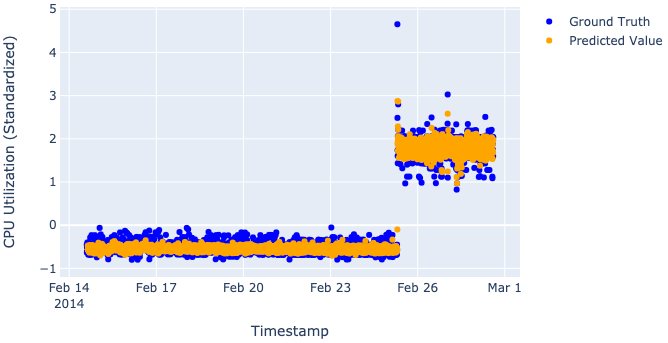
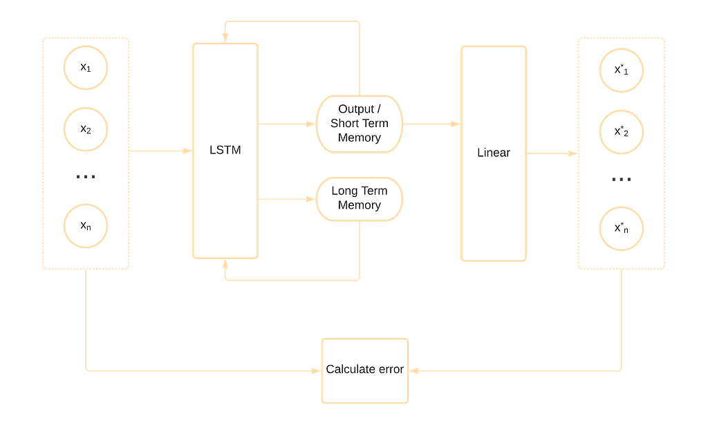
It is logical that during nighttime and daytime CPU usage may vary which is totally normal behavior. To consider this behavior, we can think of night and day times as separate “seasons”. And because of this, we will use SARIMAX — which is just a modified ARIMA model with the same idea that adds seasonal causes into ARIMA. SARIMAX will deal with the separation of seasons for us, so we don’t have to provide anything else except our dataset.

Here you can see the schema for the training process of SARIMAX:

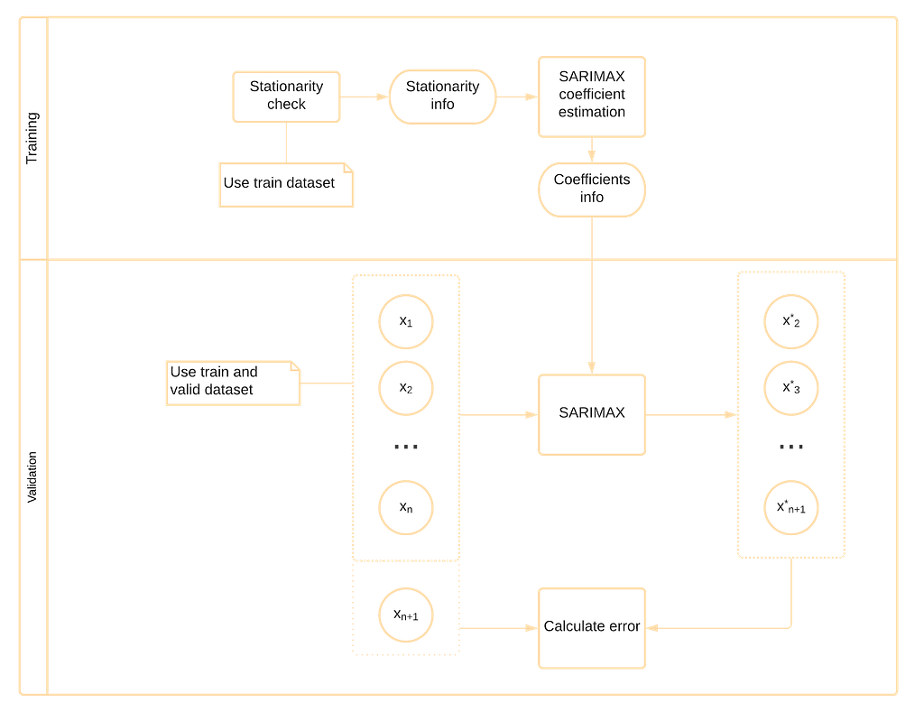
The model tries to predict the next value using the current one and then it compares the predicted result with actual value.

SARIMAX Implementation

Implementation of this model is not so interesting since all we can play with are hyperparameters for this model. To find the model that produces the best predictions we will iterate over hyperparameters and will pick the combination.

All we need is just the model itself from the statsmodels.api package and product function from itertools for iteration over hyperparameters.

And also, it would be a good idea is to write predictions of the best model into the new column of the DataFrame with initial data to ease further metrics calculation.

Here is the code to pick the best model and write its predictions into training and validation DataFrames:

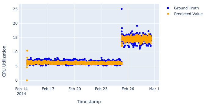
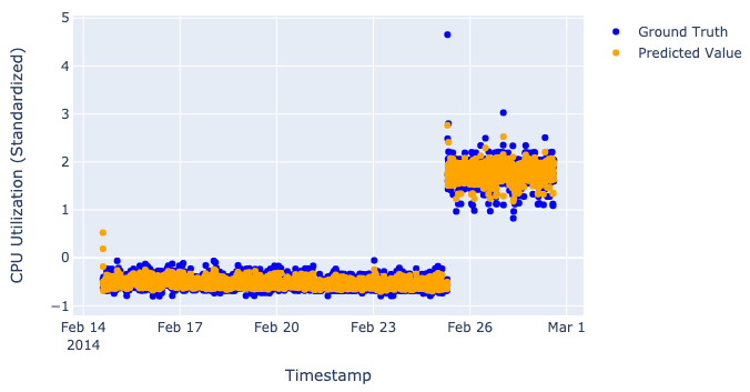
At this very moment, we have the best set of parameters and predictions for both training and validation data. To understand how good our model is, we should calculate different metrics such as precision, recall, and F-score. We will fully cover the metrics theme in Part III, however, we already can visualize the predictions and see how our model performs:

Note: one important thing about ARIMA is that time for training and optimizing the coefficients takes ~10 times longer than it takes to complete the same training of both neural networks.

Convolutional Neural Network

Convolutional neural networks are usually applied to image-connected tasks, such as image classification, segmentation, etc. But the purpose of the convolutional layers is to find and recognize patterns, which is totally applicable for analysis of the CPU utilization metric.

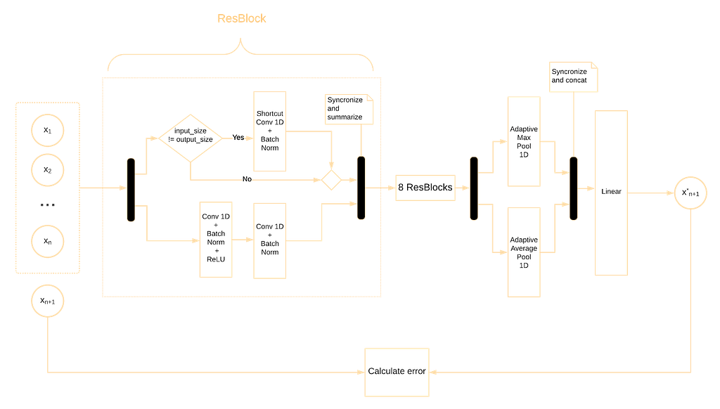
We use ResNet-ish architecture (which has already become the best type of architecture to use in CNNs) that consists of Residual Blocks (ResBlocks). The idea behind ResBlock is simple yet efficient — add the input of the block to its output. This idea allows neural networks to “remember” each intermediate result and take it into account in the final layers.

CNN tries to predict the next value using some number of previous values. In our case, this number equals 10, but of course, it may be configured.

CNN Implementation

Before coding CNN itself we should make a few additional preparations of the data. In general, since we use PyTorch, the data should be wrapped into something compatible with PyTorch’s Dataset. This may be as well the class inherited from the Dataset class, a generator, or even a simple iterator.
We will use the class option due to its readability and implicit PyTorch’s enhancements.

Once again, there are some necessary imports for Dataset creation:

Let’s recall the task for CNN. We want the model to predict the next value using some amount of the previous values. This means that our Dataset class should contain each item in a specific format — divided into 2 parts:

1. n values in sequential order that the model uses for prediction (to easily change the amount of these values, we make n the parameter)
2. 1 value that goes next after n values from the first part of the item

Coming back to the implementation — actually, it is very easy to wrap data with our custom class that just inherits from PyTorch’s Dataset. It should implement only __init__, __len__ and __getitem__ methods:

Now it is the right time to define the number of previous values that are to be used for the prediction of the next one. And, of course, wrap the data with our CPUDataset class.

Here comes the best part — the definition of the neural network.

Let’s rewind how Residual block looks like in regular ResNets. It consists of:

• Convolution layer
• Batch Normalization
• ReLU activation

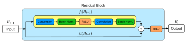
The only difference between the regular ResBlock and ours is that we removed the last ReLU activation — it turned out that in our case CNN without the last ReLU in ResBlock generalizes better.

Many Residual Blocks bring twice more Convolution + Batch Norm. (+ ReLU) combinations. So, such a combination is a good starting point to define.

In each Residual Block, we should remember about the case of changing the number of output channels (when in_feat != out_feat). One possible way to synchronize the number of channels is to multiply or cut them. However, there is another greater way — we can handle this using a 1×1 convolution without padding. This trick not only allows us to fit layer input into layer output but also adds more reasonable computations for the neural network.

It is widely used to finish the base block of the convolutional net with Max Pooling or Average Pooling depending on the task. Here comes another useful trick for Convolutional Neural Nets (thanks to Jeremy Howard and his fantastic fast.ai library) — concatenate Average Pooling and Max Pooling. It allows our neural net to decide, which approach is better for the current task and how to combine them to get better results:

And here is our resulting CNN class that is made of the building blocks that we implemented above:

Now we have the definition of CNN and can create a randomly initialized model, pass items from our Datasets, and check that data shapes are correct and that no exceptions are raised.

After the model is defined, we can move to the training loop. This loop is quite general and may be used with the majority of the neural nets:

• Loop over the epochs
• Loop over the training part of the dataset making optimization steps
• Loop over the validation part of the dataset
• Calculate losses for each epoch

Alright, we are almost ready to start fitting our CNN model. The only thing left is to initialize the model, dataloaders, and training parameters.

Here we use:

• Adam optimizer — one of the best general optimizers.
  If you have no idea which type of optimizer to pick — use Adam. Other optimizers such as SGD, RMSProp, etc. may converge better in some specific situations, but it is not our case.
• Learning rate scheduler with One Cycle policy to speed up the convergence of the neural net.
  Instead of keeping the learning rate with the same value across all iterations, we can change it. There a lot of policies such as Cosine, Factor, Multi-Factor, Warmup, etc. We choose One Cycle policy because it seems logical for us — warm-up learning rate for the ~1/3 of the iterations and then gradually decrease it.
• Mean Squared Error loss criterion as we described in Part I.

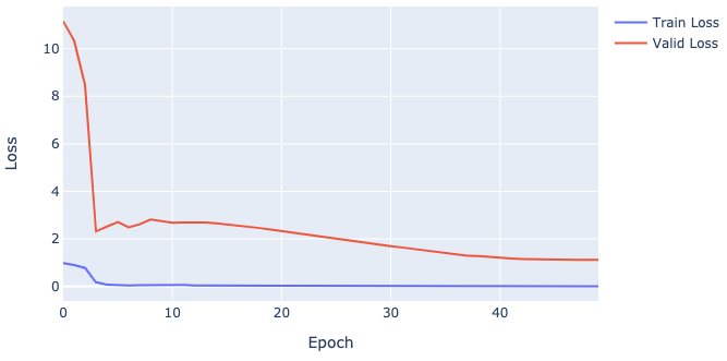
Eventually, we can run the most desired line of code — execution of the training process:

And see the losses of our model.

We always want both training and validation losses to move down because this behavior means that the model has learned something useful about our data. If any loss eventually moves up, then the model can’t figure out how to solve the task, and you should change or modify it.

These losses on the picture above seem pretty nice because they eventually move down, but it is an early assumption (their niceness) since we haven’t checked the predictions yet.

At this very moment, we can easily calculate them with our model:

And take a look:

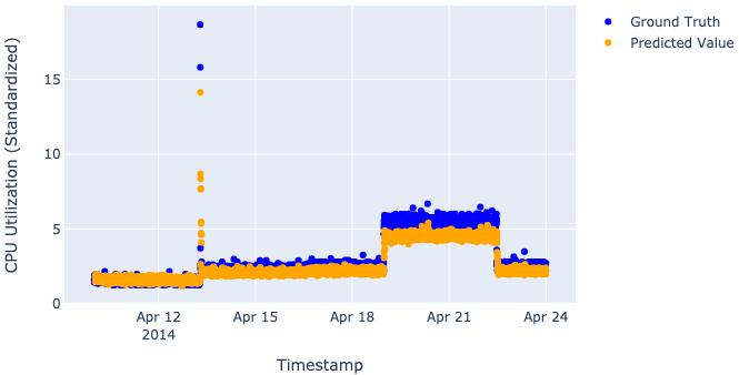
Just to be clear, we don’t really want our models to perfectly predict values, as such perfection would destroy the whole idea of the anomaly detection process (described in “Saying what we want from our models out loud” in Part I). That’s why when we look at plots, we want to see our model catch the main trend, not the particular values.

Long Short-Term Memory Neural Network

LSTM neural networks have an internal memory state that allows them to remember its’ previous evaluations that make this architecture the perfect candidate for time series anomaly detection.

Unlike the previous two models, this neural network tries to reconstruct the current value using the value itself. It may seem trivial, but this approach has extremely good results in anomaly detection.

LSTM Implementation

We can simplify the wrapping of data into the Dataset from CNN because we need the very same output as input for reconstruction. That is why we get rid of the first part of each item and just keep 1 value. We also should consider that LSTM models usually can’t be fed with the whole sequence at once (because of the memory consumption for the whole sequence)— we have to separate data accordingly into partial sequences to train. Moreover, as training with the whole sequence may reduce the model’s ability to generalize, it may simply get used to the data this way.

The definition of the LSTM neural net is much easier than the CNN one. PyTorch already has an implemented class of LSTM cells that we can use.

Considering that we changed the Dataset class a bit we also should change the training loop to fit data.

In LSTM case we also use:

• Adam optimizer
• Learning rate scheduler with One Cycle policy
• Mean Squared Error loss criterion

One more time we face the most desired line of the code with its result:

Because of the training with partial sequences, we can’t directly send the Dataset instance to get the results, but we certainly can extract the entire sequences from DataFrames:

And then we calculate the predictions:

Another intermediate conclusion

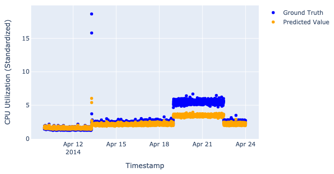
Terrific, we have 3 trained models and their results on our dataset!

The toughest part is behind us and now we are prepared to make our final steps towards anomaly detection. In the last chapter, we will do some extra preparations and reveal the detection process along with its results.

If you want to refresh some theory or data preprocessing, don’t be shy and go to the first part:

• Part I — Intro to Anomaly Detection and Data Preparation

Otherwise, the third part awaits (this item will become link like the one from the header):

• Part III — Eventually easier than it seemed

About us

We at Akvelon Inc love cutting edge technologies in mobile development, blockchain, big data, machine learning, artificial intelligence, computer vision, and many others. This article is the result of one of many projects developed in our Office Strategy Labs where we’re testing new technologies and approaches before delivering them to our clients.

If you would like to work with our strong Akvelon team — please see our open positions.

Designed and implemented with love in Akvelon:
Team Lead — Artur Khanin
Delivery Manager — Sergei Volynkin
Technical Account Manager — Max Kostin
ML Engineers — Irina Nikolaeva, Rustem Saitgareev

Don’t forget to give us your ? !

Time Series and How to Detect Anomalies in Them — Part II was originally published in Becoming Human: Artificial Intelligence Magazine on Medium, where people are continuing the conversation by highlighting and responding to this story.

Via https://becominghuman.ai/time-series-and-how-to-detect-anomalies-in-them-part-ii-bde9e69d0aaf?source=rss—-5e5bef33608a—4

Via https://becominghuman.ai/using-ai-to-win-in-love-a-step-by-step-guide-fd5eb169642a?source=rss—-5e5bef33608a—4

How to evaluate the Machine Learning models? — Part 4

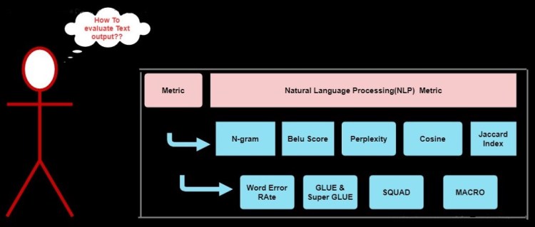
This is the fourth part of the metric series where, we will discuss about evaluation of the ML/DL model using metric NLP model are little tricky to evaluate because the output of these model is text/sentence/paragraph. So, we have to check the syntactical, semantic and well as the context of the output of the model So we uses different types of techniques to evaluate these model.

Before we start to dig deep, lets have some basic intuition about NLP model. NLP deals with Natural Language Processing i.e. it deals with the text data. We all know that ML model take input as numerical value i.e. numeric tensor and give numeric output. So we need to convert these text data into numerical format for this we have various preprocessing techniques such as Bog of Words. Word2vector, Doc2vector, Term Frequency(TF), Inverse Term Frequency(ITF), Term Frequency-Inverse Term Frequency(TF-IDF) or you can do manually by various techniques. For now you don’t need to get carried away just assume that Text have been converted by some algorithm or method into numerical value and vice versa.

Trending AI Articles:

1. How to automatically deskew (straighten) a text image using OpenCV

2. Explanation of YOLO V4 a one stage detector

3. 5 Best Artificial Intelligence Online Courses for Beginners in 2020

4. A Non Mathematical guide to the mathematics behind Machine Learning

1. N-Gram

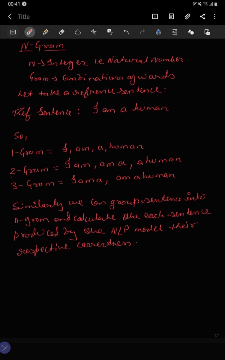
In ML gram is refers as word and N is an integer. So N-gram refers to the count of words in a sentence, if a sentence is made-up of 10 words it will be called as 10-gram. It is used to predict the probability of the next word in the sentence depending how the model is trained i.e. om Bigram trigram and so on using the probability of occurrence of the word related to its previous word.

Jupyter Notebook Link

2. BELU Score

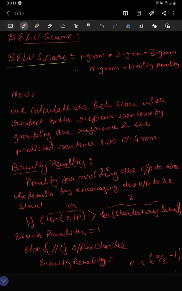
BELU stand for the BiLingual Evaluation Understudy — it was invented to evaluate the language translation from one language to another.

Steps to calculate BELU are as follows:

Step 1: From the predicted word assign the value 1 if the word matches with the training set else assign 0.

Step 2: Normalise the count so that it is has range of [0–1] i.e. total count/no. of words in reference sentence.

BELU with N-grams

As I have mentioned that we assign 1 if the predicted word matches with the training set and there is a case where the words are repeated and it can have have BELU score of 1. In this case we use combination of the words i.e. N-gram to extract the order or the word in sentence. We also limit the number of times to count each word based on the highest number of times it appears in any reference sentence, which helps us avoid unnecessary repetition of words. Finally, we try to mitigate the loss of detail in the sentence produced by the sentence at least equal to the reference sentences or sentence in the training or larger than it set by introducing brevity_penality.

Problem with the BELU Score are as follows:

1. It does not consider meaning.
2. It does not consider sentence structure.
3. It does not handle morphological rich language.

Jupyter Notebook Link

3. Cosine

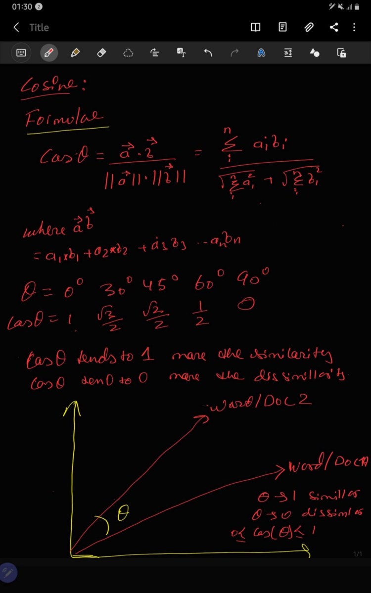
It is a metric which is used to define the similarity between two documents earlier commonly used approach which was use to match similar documents is based on counting the maximum number of common words between the documents. But this approach has flaw i.e. the size of the document increases, the number of common words tend to increase even if the two documents are unrelated. As a result cosine come into existence which removed the flaw of “ count the common word or the euclidean distance.

Mathematically, cosine is the measurement of the angle between two vectors projected in a multi-dimensional space. In this context with the NLP, the two vectors arrays of word counts of associated with the two documents. Cosine calculate the direction instead of the magnitude where as the euclidean distance calculate magnitude. It is is advantageous because even if the two similar documents are far apart by the Euclidean distance because of the size (like, the word ‘cricket’ appeared 50 times in one document and 10 times in another) they could still have a smaller angle between them. Smaller the angle, higher the similarity.

Projection of Cosine Similarity is shown below:

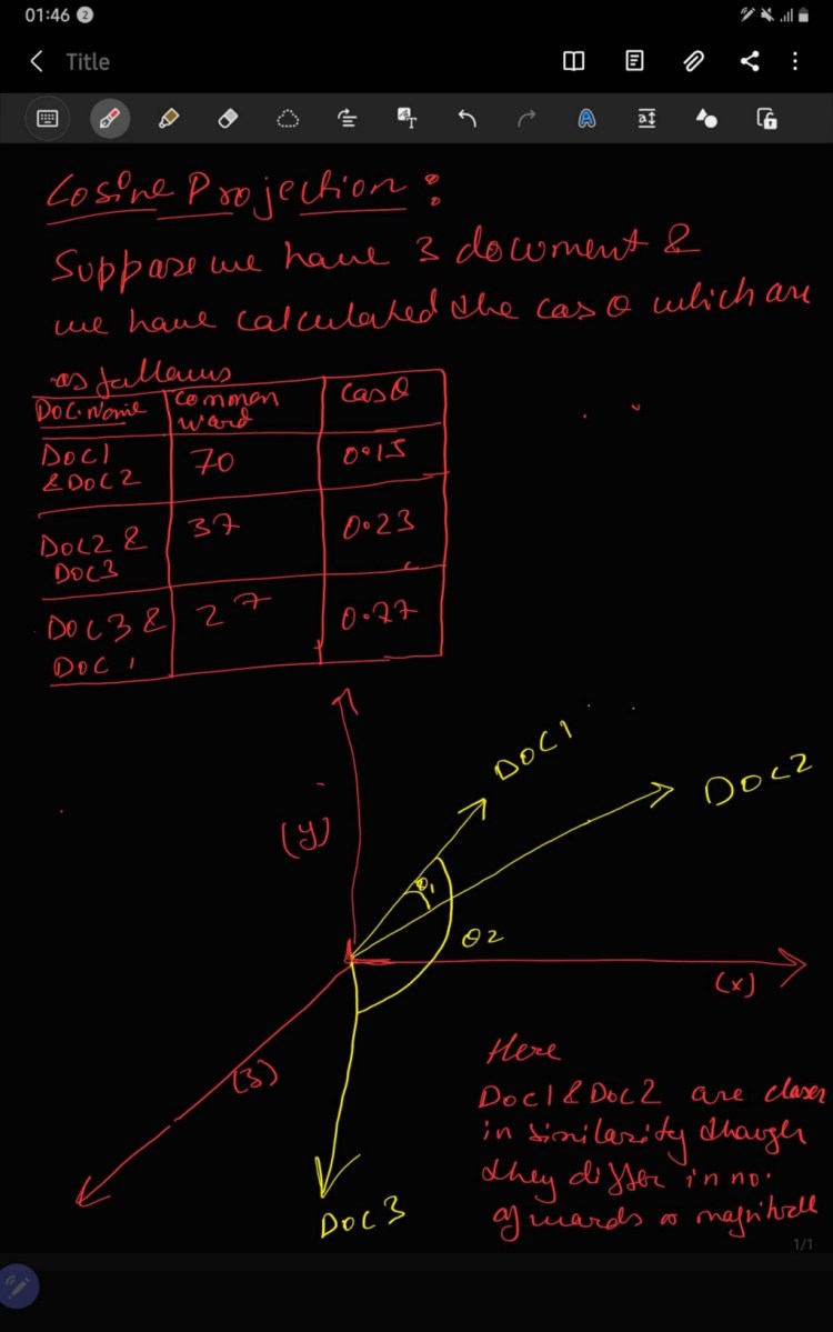
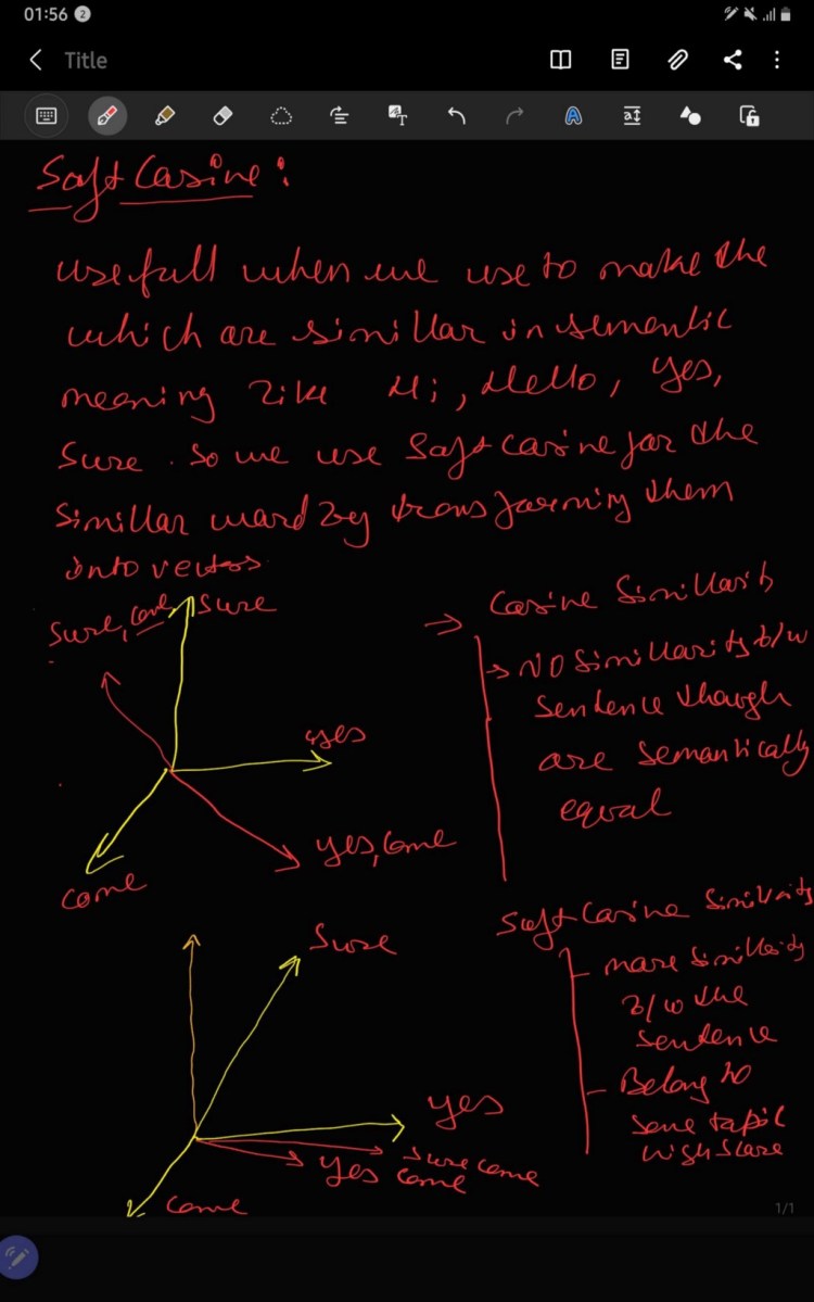
Suppose if you have another set of documents on a completely different topic, say ‘food’, you want a similarity metric that gives higher scores for documents belonging to the same topic and lower scores when comparing docs from different topics. So we need to consider the semantic meaning i.e. words similar in meaning should be treated as similar. For Example, ‘President’ vs ‘Prime minister’, ‘Food’ vs ‘Dish’, ‘Hi’ vs ‘Hello’ should be considered similar. For this, converting the words into respective word vectors, and then, computing the similarities can address this problem by soft cosine.

Jupyter Notebook Link

4. Jaccard Index

Jaccard Index is defined as the Jaccard similarity coefficient — used to understand the similarity or diversity between two finite sample set and have range [0, 1]. If the data is missing in the sample set it is replaced by zero, mean or the missing data is produced by the k-nearest algorithm or Expectation Maximisation Algorithm (EM algorithm).

Jupyter Notebook Link

5. Word Error Rate (WER)

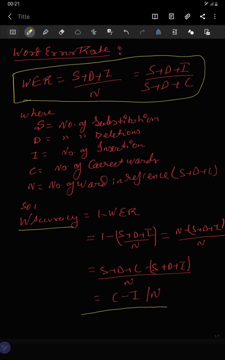
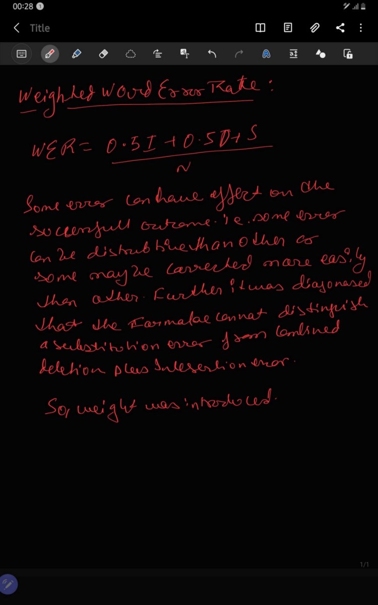
WER is derived from the Levenshtein distance i.e. working at word level instead of the phoneme level. Word Error Rate is one of the most common metric use to compare the accuracy of the transcript produced by speech recognition APIs as well as machine translation system. Instead of working with the phoneme level WER work with the word level. It is very important metric when we compare one system with other system and as well as evaluating the subsystem but it does not provide the nature of translation error.

This problem is solved by first aligning the recognized word sequence with the reference (spoken) word sequence using dynamic string alignment. Examination of this issue is seen through a theory called the power law that states the correlation between perplexity and word error rate.

Jupyter Notebook Link

6. ROUGE

ROGUE stands for Recall- Oriented Understudy for Gisting Evaluation is collection of the metric for evaluation of the transcripts produced by the machine i.e. generation of summarise text and as well as the text generation by NLP model based on overlapping of N-grams.

The metrics which are available in ROGUE are as follows:

ROUGE-N: Overlap of N-grams between the system and reference summaries.

ROUGE-1 refers to the overlap of unigram (each word) between the system and reference summaries.

ROUGE-2 refers to the overlap of bigrams between the system and reference summaries.

ROUGE-L: Longest Common Subsequence (LCS) based statistics. Longest common subsequence problem takes into account sentence level structure similarity naturally and identifies longest co-occurring in sequence n-grams automatically.

ROUGE-W: Weighted LCS-based statistics that favors consecutive LCSes .

ROUGE-S: Skip-bigram based co-occurrence statistics. Skip-bigram is any pair of words in their sentence order.

ROUGE-SU: Skip-bigram plus unigram-based co-occurrence statistics.

7. NIST

NIST stands for National Institute of Standard and Technology situate in the US. This metric is use to evaluate the quality of text produced by the ML/DL model. NIST is based on BELU score -calculate n-gram precision by giving equal weight to each one where as NIST calculates how much information is present in N-gram i.e. when model produces correct n-gram and the n-gram is rare them it will ne given more weight. In simple words we can say that more weight or credit is given to the n-gram which is correct and rare to produce as compared to the n-gram which is correct and easy to produce.

Example, if the trigram “task is completed” is correctly matched, it will receive lower weight as compared to the correct matching of trigram “Goal is achieved”, as this is less likely to occur.

8. SQUAD

SQUAD refers to Stanford Question Answering Dataset. It is collection of the dataset which includes the Wikipedia article and question related to it. The NLP model are trained on this dataset and try to answer the questions. SQUAD consist of 100,000+ question answer pairs and 500+ articles from Wikipedia. Though it is not defined as a metric but it is used to judge the model usability and predictive power to analyze the text and answer question which is very crucial in NLP applications like chatbot, voice assistance chatbots etc.

The key feature of SQUAD are as follows:

1. It is closed dataset i.e. question and answer are always a part of the dataset and in series like Name of the spacecraft was Apollo 11.
2. Most of the answer i.e. almost 75% are less than or equal to 4.
3. Finding an answer can be simplified as finding the start index and the end index of the context that corresponds to the answers

9. MACRO

MACRO stands for Machine Reading Comprehension Dataset similar to SQUAD, MACRO also consist of 1,1010,916 anonymized question collected from Bing’s Query Log’s with answers purely generated by humans. It also contains human written 182,669 question answers — extracted from 3,563,535 documents.

NLP models are trained on this dataset and try to perform the following tasks:

1. Answer the question based of the passage. As mentioned above the question can be anonymized or original question. So custom or generalized word2vec, doc2vector or Gloves are required to train the model- Question Answering
2. Rank the retrieved passage given in the question — Passage Ranking.
3. Predict whether the question can be answered from the given set of passages if yes then extract and synthesize the predicted answer like a human.

Don’t forget to give us your ? !

How to evaluate the Machine Learning models? — Part 4 was originally published in Becoming Human: Artificial Intelligence Magazine on Medium, where people are continuing the conversation by highlighting and responding to this story.

Via https://becominghuman.ai/how-to-evaluate-the-machine-learning-models-part-4-7cd415be62db?source=rss—-5e5bef33608a—4