365 Data Science is an online educational career website that offers the incredible opportunity to find your way into the data science world no matter your previous knowledge and experience.
Join Metis Senior Data Scientist Kevin Birnbaum, on Nov 19 @ 12 PM ET, as he explains how spreadsheets can help all employees get comfortable with data and empower them to perform their own analysis without hand holding by your advanced analytics team.
PyCaret is an alternate low-code library that can be used to replace hundreds of lines of code with few words only. This makes experiments exponentially fast and efficient. Find out 5 ways to improve your usage of the library.
Time Series and How to Detect Anomalies in Them — Part I
Intro to Anomaly Detection and Data Preparation
Hello fellow reader, my name is Artur. I am the head of theMachine Learningteam inAkvelonand you are about to read the tutorial for anomaly detection in time series.
During our research, we’ve managed to gather a lot of information from tiny useful pieces all over the internet and we don’t want this knowledge to be lost! That’s exactly why you can exhale and dive into these end-to-end working articles.
The next part of the series is already published! Check it out after this one (or if you want to go straight to the models):
1 more part is coming very soon, stay in touch and don’t miss it! This item will become a link to the next chapter:
Part III — Eventually easier than it seemed
Let’s get this started!
Artificial Intelligence Jobs
First of all, let’s define what an anomaly detection problem is in general
Anomaly Detection— is the identification of rare items, events, or patterns that significantly differ from the majority of the data.
Well, basically, the anomaly is something that makes no or little sense when you look at it from the high ground.
“It’s over, Anakin. I have the high ground.” scene from Star Wars: Episode III — Revenge of the Sith
And it brings us to the fact that anomalies are extremely context-dependent. And also, different people may consider different pieces of data as anomalies.
Why do we bother finding anomalies?
Imagine the situation — you are the Co-founder and CTO in a small startup company. Your company has 1 web application and every single client really matters for success. One day a smart client found the backdoor in your app and started to send direct large queries to your database. The CPU usage has changed because of these queries but it stayed in normal boundaries.
The data may leak for a very long period of time, and when somebody else will find this backdoor and make it public, it may cause enormous damage. And this situation is not about the code quality, there is always the risk that mistakes and backdoors may appear in your app and codebase. This situation is about the drawing of your attention (as CTO and one of the main decision-makers) to reveal the issue and save your business.
Generally speaking, if you can notice any variations of your system from its normal behavior, you can find out the reasons for such behavior, uncover and eliminate hidden issues and find new non-obvious opportunities.
However, it is quite expensive to hire someone for monitoring all your metrics 24/7. That is why we want to detect unexpected variations (anomalies) automatically, inexpensively (also in terms of damage), and quickly.
Alright, now we know why we want to solve this problem. But before moving to the how part, we need to distinguish between generic anomalies and anomalies in time series. This will help us to understand what types of techniques are more appropriate for our problem.
Generic anomaly detection
Here is a generic example, which illustrates the cluster-based approach. Shortly speaking, the cluster-based approaches try to group similar data in clusters and consider values that don’t fit in these clusters as anomalies.
Example of 2D data with anomalies found via clustering
Although this picture illustrates some specific approach, the idea is the same across any technique used. We have some values with no particular order and we try to figure out which values seem uncommon.
Time series anomaly detection
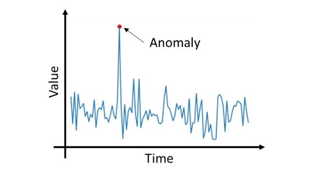
On the other hand, when we talk about anomaly detection for time series, the value itself may not seem suspicious, but it becomes suspicious due to the time when it appears and the values before:
Example of the time series with an anomaly
For example, it is okay, when the CPU load of some application is about 20%, but it seems strange when the load unexpectedly jumps to 80%. And one more important thing is that the load level around 80% after this jump is not suspicious anymore. That is why some threshold warning values can’t handle such complex situations.
The moment of the jumpis way more important than the stabilization after it.
When you’re dealing with the anomalies in general, you can shuffle them into any order and the anomalies will still be the same. If a person bought 1000 packs of toilet paper, you probably will always say that this seems anomalous.
When you’re dealing with the anomalies in time series, the order of data is important. If nobody ever bought a single pack of toilet paper in a particular store, and then a person bought just 1 pack — you already should consider it as an anomaly.
Cool, now we are ready to move on to the how part!
How to find anomalies
The general idea
One of the most common and the most successful yet approaches can be described as:
Find out what is normal and if something deviates too much from it — this is an anomaly.
And almost all of the approaches listed below try to achieve this one way or another.
Possible Approaches
Here are the most common approaches to use for anomaly detection:
These are just some of the popular techniques amongst the possible ones.
How we find anomalies
Of course, every technique listed above can be used for our purposes. But nowadays, neural networks are in trend and outperform classical algorithms almost everywhere. After our research, we decided to try 2 types of neural networks and took 1 classic model as a baseline for comparison. And here is why:
ARIMAstatistical model as a baseline — this is the classic auto-regression model that is made exactly for the time series
Convolutional Neural Network— such neural networks are usually used for image processing, but if you dig deeper into them, you may find that they actually look for the patterns in the images. Our time series also consists of patterns
And for the development we chose this set of tools:
Jupyter Notebooks environment for the implementation of the models. We prefer using Jupyter Notebooks instead of regular editors (such as JetBrains’ PyCharm) since Notebooks save code into separate cells, which can also be run in any order you need. Most editors use .py files and execute the whole bunch of code every time you run it — this makes the code modification process terrifying (sometimes training of a model consumes hours) because you have to wait to see the outcome of your simple print function at the end of your code. Thus, cells of Notebooks provide flexibility for Machine Learning development and make it easier to try something out.
Scikit-learn for some data preprocessing. Scikit-learn has many tools that are already implemented. There are no big secrets behind the data preprocessing, and we don’t really want to waste our time implementing them from scratch, optimizing them for large amounts of data, etc. This is where Scikit-learn comes in handy.
Statsmodel library for ARIMA model. This library is used with the same motivation as scikit-learn. No big secrets behind ARIMA; already implemented tool; no need to waste time.
PyTorch for neural networks. It is one of the most used libraries for the construction of neural nets. The alternative is, of course, Tensorflow. They both have pros and cons and we choose PyTorch because it is designed for eager execution that is way more flexible. On the other hand, Tensorflow is designed for building the whole calculation graph with the training/validation phase, metrics calculation, etc., meaning that a lot of stuff has to be done before. For example, you may face some syntax error at the very beginning of a model definition right after you finish coding the whole model.
Plotly for plots and graphs. When we just started, we decided to use Matplotlib, which is used almost everywhere for plots and graphs. However, we’ve noticed a new player — plotly — and it turned out that it plots prettier and more informative graphs with less code.
Before diving into models architecting and implementation we should load the data and inspect it.
Dataset Loading
First of all, we should choose the dataset for our experiments. The internet is full of different datasets, for example, you can use Dataset Search from Google to find the appropriate one. We already have the perfect repository for time series anomaly detection — The Numenta Anomaly Benchmark (NAB):
NAB contains many files with different metrics from different places. It is in the nature of metrics — being ordered in time and thus, being one of the best candidates for time series anomaly detection.
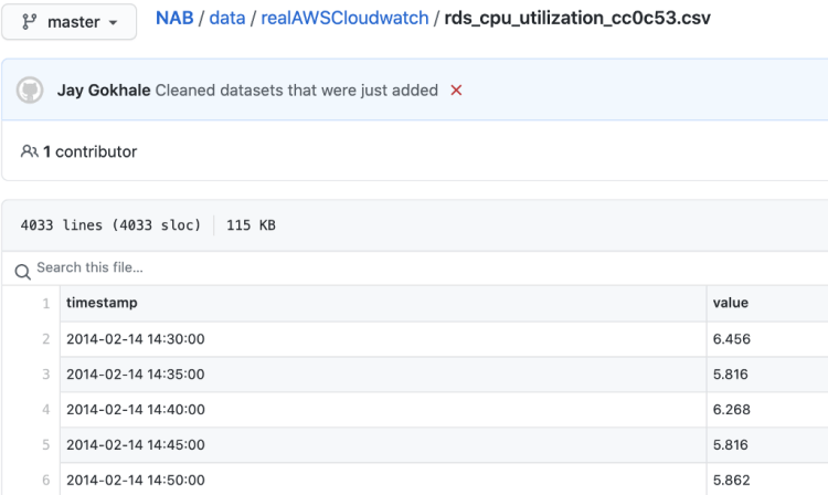
From NAB we decided to use Real CPU utilization from AWS Cloudwatch metrics for Amazon Relational Database Service. These metrics are saved in csv format and the exact timestamps of anomalies in them (let’s call itlabels) are saved in json format. You may use any other metric that you like.
Just to clarify — these anomalies that we see in the dataset were marked as anomalies by the creators.
Here are direct links to the files in NAB that we use, you can download them, take a look and play around:
The dataset is chosen, great! Certainly, you can pick any other dataset, but we will focus on NAB. Next steps that we should do:
Go through the README file from NAB repository to understand what we are working with
Load data into our local filesystem
Inspect our data of interest visually with anything that can open csv and json. Actually, we can directly open them in GitHub repo
Load data into our notebook’s environment to make further manipulations inside the notebook using Python. We use Pandas and NumPy libraries— pretty standard choice for data loading and manipulation already has several tools that have been implemented
Assuming that we already went through the README, we can move to the loading into our local filesystem.
This dataset is located in git, but it doesn’t mean that every dataset should be version controlled. We need just csv with data and json with anomaly labels and they can even be simply on the local hard drive. Git here is for convenience. Let’s grab the data into our local environment to manipulate them any way we want:
After some initial inspection in NAB’s GitHub repo, we see that both training and validation files consist of timestamps with corresponding values.
Header and first 5 rows in the training fileHeader and first 5 rows in the validation file
Each file contains 4032 ordered data rows with a 5-minute rate.
Let’s find these files in labels (once more,json with exact timestamps of anomalies).
Timestamps of the anomalies for both training and validation data from the file with labels
We can see that each file contains 2 anomalies.
Since we know what we are dealing with, we can start loading into the notebook with imports of some useful packages:
We already downloaded training and validation files and the file with labels via git. But we also downloaded all other files from the repository, so we need to specify paths to our data of interest:
Finally, we can load timestamps for anomalies from json into our local environment:
And read our data with pandas into DataFrame object:
Result of train.head()
As you can see, we’ve managed to load data and take a look at the first 5 rows from the training file. It is enough to understand that we succeeded — these rows are exact 5 first rows that we saw on GitHub.
Data Preprocessing
Great, we’ve loaded data into our notebook and inspected it a bit, but are we good to go with it and move on to the models part? Unfortunately, the answer is no.
We have to define exactly what part of the loaded data exactly will be used by our models. We have to think about the problem we want to solve and what data can be used for this.
In our case, we want to detect anomalies in CPU usage. Well, here is the answer, the clearest choice is value column because it represents CPU usage.
We also can consider timestamp column — a timestamp encodes a lot of information, i.e. what day of the week it is, what month of the year it is, etc. This information can be extracted and used by the models. We won’t do it in this article, but if you want, you can try it. Maybe, you’ll achieve even better results!
So, we are going to use value column from training and validation DataFrames. The next step is to transform values from this column into an appropriate format. The appropriate format, as you might guess, is numbers. This comes from history — computers use numbers for calculations (and ML models as well), you have to make everything numbers, it’s just the way it works.
Luckily, value column already consists of numbers, and we can use them in our models as it is. But it is pretty often a good idea to standardize numbers before feeding our models with data. It helps them generalize better and avoid problems with different scales of values with different meanings (Yes, somebody tried it in ML and it worked). Quite often standardization just means rescaling the numbers to mean= 0 and standard deviation= 1.
That’s why the next thing we have to do is to parse datetime from timestamps (just for convenient visualization) and standardize values.
We will follow the regular rescaling policy (as we said — mean = 0 and standard deviation = 1) and use StandardScaler from Scikit-learn:
Then we can extract anomalies into dedicated variables for both training and validation data from DataFrames:
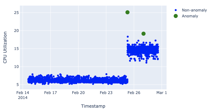
And plot all data with the help of the Plotly library to visualize the whole set of data points and gain more understanding of what it present.
Firstly, we plot the training data. (We are going to use this code for plotting everything we need)
Secondly, we plot the validation data.
I suppose this blue annoying dot between 60 and 70 needs an explanation — why isn’t it marked as an anomaly? The thing is that this dot goes right after the green anomaly dot between 70 and 80. And after ~77% of CPU load, ~67% doesn’t seem suspicious at all. You also should keep in mind that we can’t look ahead because real data comes in real-time so what looks like an anomaly at some one moment may not look like an anomaly in the full picture.
You may notice that at this moment you feel much more comfortable with data. That usually happens due to visual inspection of data values, so it is strongly advised to visualize and examine it with your own eyes.
Saying what we want from our models out loud
Now we know what our data looks like and what kind of data we have. We don’t have much information, actually, just timestamps and CPU loads. But still enough to build quite great models.
So, here comes the best moment to ask a question — “How our models are going to detect anomalies?”
To answer it we need to figure out 3 things (remembering the general idea of the anomaly detection and that our data are time series):
What is normal? This question can enforce your creativity because there is no strict definition of normality. Here is what we came up with (like many other people). We will use 2 almost identical tasks to teach our models “the normality”: 1. Given the value of CPU usage, try to reconstruct it. This task will be given to the LSTM model. 2. Given the values of CPU usage, try to predict the next value. This task will be given to the ARIMA and CNN models. If the model reconstructs or predicts easily (meaning, with little deviation), then, it is normal data. You can change this distribution of the tasks for models. We tried different combinations and this one was the best for our dataset.
How to measure deviation? The most common way to measure deviation is some kind of errors. We will use the squared error between the predicted value (x*) and the true one (x). Squared error = ❨?*−?❩² For ARIMA we will use absolute error =|?*−?|since it performed better. The absolute error may also be used in other models instead of the squared error.
And what is “too much” deviation? Or in other words how to pick the threshold? You can simply take some numbers or figure out some rules to calculate it. We are going to use the three-sigma statistic rule by measuring the mean and the standard deviation of the errors in all training data (and only training, because we only use validation data to see how our model performs). And then we will calculate the threshold, above which deviation is “too much”. And, looking ahead, we will also use a slightly modified version with measuring over some window behind the current position to incredibly enhance accuracy.
Don’t worry, if it seems too complicated right now, it will become much more clear, when you will see it in the code.
Intermediate conclusion
Great, most of the theory part is done, and we have loaded, inspected, and standardized our dataset!
As the practice shows, data preparation is one of the most important fragment sand. We will prove this in the further parts because the code that we implemented here is a strong fundament that we will use in all our models.
And very soon you will be able to move forward (these items will become links like the ones from the header):
We atAkvelon Inclove cutting edge technologies in mobile development, blockchain, big data, machine learning, artificial intelligence, computer vision, and many others. This article is the result of one of many projects developed in our Office Strategy Labs where we’re testing new technologies and approaches before delivering them to our clients.
Graph neural networks (GNNs) belong to a category of neural networks that operate naturally on data structured as graphs. Despite being what can be a confusing topic, GNNs can be distilled into just a handful of simple concepts.
Starting With Recurrent Neural Networks (RNNs)
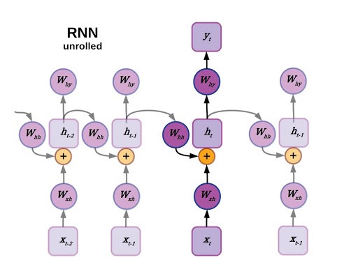
We’ll pick a likely familiar starting point: recurrent neural networks. As you may recall, recurrent neural networks are well-suited to data that are arranged in a sequence, such as time series data or language. The defining feature for a recurrent neural network is that the state of an RNN depends not only on the current inputs but also on the network’s previous hidden state. There have been many improvements to RNNs over the years, generally falling under the category of LSTM-style RNNs with a multiplicative gating function between the current and previous hidden state of the model. A review of LSTM variants and their relation to vanilla RNNs can be found here.
Unrolled RNN.
Although recurrent neural networks have been somewhat superseded by large transformer models for natural language processing, they still find widespread utility in a variety of areas that require sequential decision making and memory (reinforcement learning comes to mind). Now imagine the sequence that an RNN operates on as a directed linear graph, but remove the inputs and weighted connections, which will be embedded as node states and edges, respectively. In fact, remove the output as well. In a graph neural network the input data is the original state of each node, and the output is parsed from the hidden state after performing a certain number of updates defined as a hyperparameter.
Artificial Intelligence Jobs
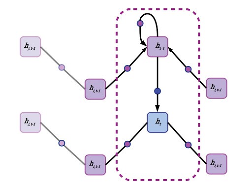
Reimagining Recurrent Neural Network (RNN) as a Graph Neural Neural Network (GNN)
Re-imagining an RNN as a graph neural network on a linear acyclic graph.
First, each node aggregates the states of its neighbors. This can be accomplished by forward passes through a neural network with weights shared across edges, or by simply averaging the state vectors of all adjacent nodes. A node’s own previous hidden state is also included in this neighborhood aggregation, but often gets special treatment. A node’s self-state may be parsed through its own hidden layer or by simply appending it to the state vector aggregated from the mean of all neighboring states. There’s no concept of time in a generalized GNN, and each node pulls data from its neighbors regardless of whether they are “in front” or “behind,” although in a directed graph or graph with multiple species of connections, different edges may have their own aggregation policies. Another term for neighborhood aggregation is neural message passing.
It’s easy to get bogged down in the details, and there’s quite a bit of room for versatility in GNNs.
In general, GNN updates can be broken into two simple steps:
Aggregate or parse states of neighboring nodes, aka “message passing.”
Update node state
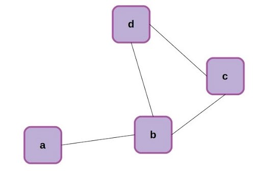
Now that we’ve made the connection that an RNN can be formulated as a special case of a graph neural network, let’s back up for a moment and make sure we’re all familiar with the same terms. Graphs are a mathematical abstraction for representing and analyzing networks of nodes (aka vertices) connected by relationships known as edges. Graphs come with their own rich branch of mathematics called graph theory, for manipulation and analysis. A simple graph with 4 nodes is shown below.
Simple 4-node graph.
The nodes of the above graph can be readily described as a list: [0,1,2,3], while the edges can be described as an adjacency matrix, where each edge is represented by a 1 and missing connections between nodes are left as 0.
Non-Directed Nature of GNNs
The adjacency matrix above reflects the non-directed nature of the corresponding graph. A connection between node 0 and node 1 is the same type of connection as that between 1 and 0, and this is reflected in a symmetry about the matrix diagonal. It’s also not unusual to reflect node self-connections in the adjacency matrix, and we can easily update the matrix to show this by adding the identity matrix of equivalent size, giving the adjacency matrix a value of 1 at every diagonal element.
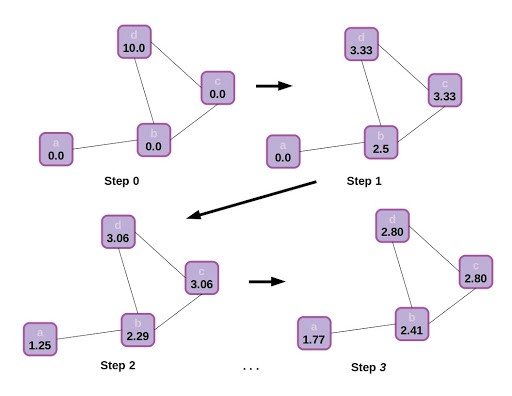
Just to build a final bit of intuition, let’s visualize how information propagates through the graph. In this case there is no step 2 for updating node states (or we can think of the update step as being an identity function), and node states are represented by scalars.
State propagation or message passing in a graph, with an identity function update following each neighborhood aggregation step. The graph starts with all nodes in a scalar state of 0.0, exceptingdwhich has state 10.0. Through neighborhood aggregation the other nodes gradually are influenced by the initial state ofd, depending on each node’s location in the graph. Eventually the graph will reach equilibrium and each node will approach a scalar state value 2.5.
That simple example of scalar state propagation in a graph gives us an intuitive feel for how the structure of a graph affects information flow, and how this might affect the final output of the model. It makes sense that nearby nodes will have a greater effect on one another than distant ones, and influence will be impeded by traveling through sparse connections.
What Does This Mean for the Adjacency Matrix?
Returning to the adjacency matrix mentioned earlier: that’s actually an especially easy way to aggregate the states of neighboring nodes. We can simply matrix-multiply the array of node states by the adjacency matrix to sum the value of all neighbors, or first divide each column in the matrix by the sum of that column to get the mean of neighboring node states. That’s an easy and computationally fast way to define and implement neighborhood node aggregation.
Another strategy is to define each type of edge as a feed forward neural network, sharing weights with all the instances of that type of edge. The feed forward network is applied to each neighbor node state vector before averaging, or, in a graph attention network, applying attention and then summing. Finally, in a real GNN, after aggregating state data from a node’s self and neighbors, the node’s state is updated. The update rule can be any type of neural network, but it’s common to use a recurrent model like a gated recurrent unit (GRU).
Applying Graph Neural Networks to Useful Inference
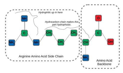
Let’s take a realistic (but still simplified) scenario amenable to applying graph neural networks, to see how this structural information contributes to useful inference. Say we wanted to predict which atoms in amino acid residues were hydrophilic (miscible in water) as opposed to those that are hydrophobic, like oils. That’s important information for determining how proteins fold, a difficult and fundamental question in molecular biology. We’ll examine arginine as an example, an amino acid with both hydrophilic and hydrophobic traits. After formulating the molecule as a graph:
Graph representation ofarginine, an amphipathic amino acid.
We can run neighborhood aggregation and state updates to get a prediction of hydrophilicity at each node. At physiological pH, the amino groups in the backbone and amino acid sidechain of arginine are protonated. On the other hand, the long hydrocarbon chain connecting the backbone to the end of the side-chain is very hydrophobic, so arginine has both water-loving and water-repelling characteristics.
An interesting aspect of the arginine side-chain that affects this dual nature is that the hydrophilicity is distributed across all three nitrogen-containing amino residues in the side-chain. The term for this arrangement of 3 nitrogens around a central carbon is a guanidino group. It’s hard to imagine capturing this distributed hydrophilicity by considering each node in isolation, but it’s exactly the type of insight that can be learned by incorporating the structural information of a graph.
A Tour of Graph Neural Network Applications
Although graph neural networks were described in 2005, and related concepts were kicking around before that, GNNs have started to really come into their own lately. In the last few years, GNNs have found enthusiastic adoption in social network analysis and computational chemistry, especially for drug discovery. As such it’s not a bad time to get familiar with the promising style of model in case you may run into those types of problems that can be readily formulated on graphs.
Materials science has recently been an attractive area for applying GNNs. Deepmind published results earlier this year using GNNs to shed light on the glass transition, a subject of substantial contention in physics. That’s part of a larger trend using GNNs to studymaterialproperties. A related application domain, and perhaps the most exciting in terms of potential impact, is graph neural networks for chemistry. GNNs are particularly well suited for neural reasoning about molecules, including the small molecules that make good drug candidates. If you are interested in working in or gaining a better understanding of machine learning for drug discovery working with GNNs is practically a must-have skill.
What’s Next for Graph Neural Networks (GNNs)?
Attention is a concept that gives machine learning models the ability to learn how to apportion different weights to different inputs, in other words giving models the capability to manage their own attention. We can point to Vaswani et al.’s “Attention is All You Need” as an example of recent seminal work in this area. The paper posited the attention-only transformer as a do-it-all language model (see here for more about attention and transformers). This has for the most part held true with the development of massive transformer models like BERT and GPT-3 dominating natural language metrics in recent years.
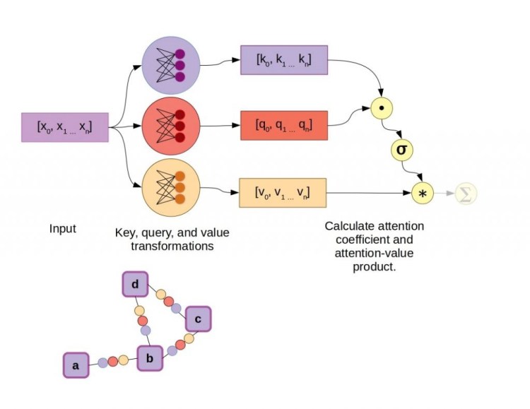
Adding attention to the existing GNN algorithm we discussed earlier is fairly simple. During neighborhood aggregation, in addition to transforming the states of neighboring nodes via a feed-forward network on graph edges, an attention mechanism is included to calculate vector weighting coefficients. Several attention mechanisms are available, such as the dot-product attention mechanism used in the original transformer models, as well-illustrated by Jay Allamar. In this scheme, fully-connected layers produce a key and query vector, in addition to a value vector for each input, which in this case are connected to nodes by graph edges. Taking the dot product of the key and query vectors yields a scalar constant, which is then subjected to a softmax activation function alongside all other key-query dot products in the graph neighborhood, aka the raw attention coefficients. Finally, instead of summing all the value vectors directly, they are first weighted by the attention coefficients.
Example of a Graph Attention Network using the dot-product attention mechanism. In this caseσrepresents the softmax function.
Quantum Graph Neural Networks (QGNNs)
If quantum chemistry on graph neural networks is an effective way to take advantage of molecular structure when making inferences about quantum chemistry, defining the neural networks of a GNN as an ansatz, or quantum circuit architecture, can bring models even closer to the system they are making predictions and learning about. Quantum graph neural networks (QGNNs) were introduced in 2019 by Verdon et al. The authors further subdivided their work into two different classes: quantum graph recurrent neural networks and quantum graph convolutional networks.
The specific type of quantum circuit used by QGNNs falls under the category of “variational quantum algorithms.” In short, these are quantum circuits with parameters that can be trained by gradient descent, and these trainable parameters are the quantum equivalent of weights and biases. A known issue in training variational quantum algorithms/circuits is the presence of “barren plateaus,” regions in the fitness landscape where the objective score doesn’t change very much. QGNNs were devised as a means of imparting structural information to variational quantum circuits to ameliorate the presence of barren plateaus. Verdon and colleagues demonstrated QGNNs applied to learning quantum dynamics, graph clustering, and graph isomorphism classification.
Replace Neural Networks with Graph Neural Networks (GNNs)?
Should you convert your datasets to graphs, and replace all of your neural networks with GNNs? The answer, of course, depends on your problem’s natural suitability as a graph. Forcing a dataset that is better represented on a linear sequence or 2D grid to fit on a graph will probably only lead to more difficult implementation and slower training. GNNs do look like they’ll be the dominant model type for machine learning on molecules for the next few years, so if you’re going to be working in computational chemistry it’s an important tool to be familiar with. That goes double for drug discovery and development.
GNNs also seem to be a good match for social media graphs and other types of relational networks naturally representable as graphs. Although GNNs have been used for image and language-based tasks, transformers and the old reliable conv-nets seem to have those areas pretty well covered for now. As a final note, GNNs also might make a compelling framework for combining deep learning neural networks with “Good Old-Fashioned AI” (GOFAI), a topic that was reviewed in a JCAI survey paper on neurosymbolic AI. This hybrid approach may offer some advantages in terms of interpretability and control, at some cost in overall flexibility.
Bringing GNNs Into the Future
If you’ve heard of graph neural networks but have been put off by their seeming complexity, hopefully this article has helped to overcome that initial hurdle. Remember, GNNs are just deep learning models that reside on and operate on graphs. There’s plenty of flexibility in how you build one, but they all share the basic steps of neighborhood aggregation followed by state updates. If you’ve been waiting to see a noteworthy commercial success before diving in, look no further than the impact of GNNs on computational chemistry and drug discovery over the next few years. It’s a worthwhile model class to be familiar with, and set to find increasing traction and impact over the course of this decade.
Ever since the evolution of Artificial Intelligence (AI), humankind had dreamt of machines that can converse in natural languages. With the suprise of Deep learning (DL) techniques, High-performance computers, and big data, that dream today appears to be closer than ever before. This article gives an overview of Natural Language Processing (NLP), its challenges, and the recent DL trends in NLP research.
What is NLP?
Natural language processing (NLP) is an interdisciplinary field of linguistics and computer science. The goal of NLP research is to design/develop efficient computational models to analyze, understand, and generate human language. Its application ranges from simple spell checkers in text editors to sophisticated chat-bots in virtual assistants like Alexa and Siri.
Artificial Intelligence Jobs
Why is it challenging?
Unlike programming languages that have fixed syntax and befitting semantic rules, human languages are inherently ambiguous. A thought can be expressed with different sets of words, arranged in multiple ways. A word can have different meanings in different contexts. A collection of words, when arranged differently, may convey the same or different thought. These challenges make natural language understanding (NLU), an exciting research topic. Over the past few decades, NLP has evolved from traditional rule-based systems to shallow machine learning models and further to Deep Neural Network models.
Deep Learning in NLP
The first step in any DL-NLP model is to convert the input text into a format that your machine learning algorithm can understand, which are vectors (or tensors). Word-embeddings are real-valued dense vectors used to represent word meaning. Word2Vec (by Google), GloVe (by Standford), and fastText (by Facebook AI) are some of the widely used word-embeddings. These word embedding are generated from the vast text corpus using shallow neural networks. The models, as well as their trained word vectors for nearly 2 million words in different languages, are freely available for download. They also have support on most DL libraries. Researchers around the globe have been trying to improve these word embeddings.
The next step is to combine these word vectors to get an abstract representation of larger text required for the task at hand. The model uses specialized deep neural network architectures, which are powerful enough to extract relevant features from these inputs and generate the desired output. Recursive Neural Networks (RNN), Long Short Term Memory Network (LSTM), Encoder-Decoder models, and Transformers are the favorite DL architectures of NLP researchers. Are there better ways to compose sentence vectors from these word embedding, is an open research problem.
In the past, NLP models were designed and trained for a single specific task and were good at only that particular task. Recently the paradigm has shifted to Transfer learning and pre-trained model. The idea behind transfer learning is to extensively train large neural networks on generalized language understanding tasks using large datasets. These pre-trained models have a general understanding of the language and can be fine-tuned for a wide variety of NLP tasks with little or no extra training. Some of the popular pre-trained models that stand out in 2020 are Google’s T5, BERT, XLNet, ALBERT, Facebook’s ROBERTa, OpenAI’s GPT-2, and Nvidia’s Megatron. Some of these models are publicly available and can be used off-the-shelf for many NLP applications. Pre-training allows researchers to work on models trained on datasets that are not accessible to the public or are computationally expensive to train.
Well-known NLP tasks used to train and evaluate a model’s language understanding include:
Named Entity Recognition (NER): Which words in a sentence are a proper name, organization name, or entity?
Recognizing Textual Entailment (RTE) / Natural Language Inference (NLI): Given two sentences, does the first sentence entail or contradict the second sentence?
Coreference Resolution: Given a pronoun like “it” in a sentence that discusses multiple objects, to which object does “it” refer?
Acceptability: Is the given sentence grammatically acceptable or not?
Sentiment Analysis: Is the given review positive, negative, or neutral?
Sentence similarity measure: How similar are the given two sentences in their meaning?
Paraphrase Identification: Is sentence B a paraphrase of sentence A?
Question NLI: Given a question-paragraph pair, does the paragraph contain the answer to the given question?
Question Answering: Does the sentence B correctly answer question A?
NLP tasks like Machine Translation and Dialogue systems require not just language understanding but also generation. Common Sense Reasoning (CSR) is also one such task recently added to the DL-NLP benchmark. Another interesting recent research topic is summarizing programming language code in natural language text. It could be useful for automatic documentation of source codes. Refer GLUE or superGLUE benchmark for more challenges, best models, and free resources.
NLP also has applications in other domains like Biomedical text mining, Healthcare, Business, Recruitment, Defence and National security, Finance, and Education, to name a few.
Tips for beginners
For beginners in DL-NLP research, I did recommend Linear Algebra and Probability and Statistics courses as prerequisites. Basic knowledge of Machine Learning and a bit more detailed understanding of Deep Learning can give you a better start. It would be good to learn Pytorch as most of the source codes published in Github are in PyTorch. If your research does not involve building any special kind of neural network, Keras is your best option. TensorFlow and Theano are also attractive choices.
Note: The article was originally published in the 2020 Yearbook edition of Threads — the official newsletter of the Computer Science and Engineering Department of NIT Calicut
Breaking into any new field or slogging through a career change is always a challenge, and requires focus and even a little grit. While transitioning to becoming a Data Scientist is no different, aspiring to this role is possible, even without a formal post-secondary degree, largely due to the vast amount of quality learning resources available today.
Also: Learn to build an end to end data science project; How to Acquire the Most Wanted Data Science Skills; Moving from Data Science to Machine Learning Engineering; Learn to build an end to end data science project; DIY Election Fraud Analysis Using Benford’s Law
This article compiles the 30 top Python libraries for deep learning, natural language processing & computer vision, as best determined by KDnuggets staff.
If machine learning models predict personal information about you, even if it is unintentional, then what sort of ethical dilemma exists in that model? Where does the line need to be drawn? There have already been many such cases, some of which have become overblown folk lore while others are potentially serious overreaches of governments.
In this tutorial, we will start with the most simple artificial neural network (ANN) and move to something much more complex. We begin by building a machine learning model with no parameters—which is Y=X.