365 Data Science

Creating ML model for News Classification

This blog will be divided into four parts. Because I will try to explain the stuff from scratch so that if you have some basic knowledge about ML and python you do not need to wander here and there for deploying your first model on the WEB. Also, these four parts are going to be published at once so no need to worry about waiting for the next part.

Part 2 — Creating News Classification Django App ( Part 1) Link

Part 3 — Creating News Classification Django App ( Part 2) Link

Part 4 — Deploying on Heroku and live on Web Link

So are you ready?

So what are we going to deploy?

I am thinking about lots of stuff to share with you guys but as a start, I thought it’s better to deploy a News Classification model on Heroku. And this project is going to be made from scratch.

In this part of the series, I will tell you how to create a News classification model and save it for further use.

If you are wondering how our Web APP looks like. Below is the .GIF of a real working app and its link. (Wait for few seconds after clicking the link)

So without any further delay. Let’s get started. 🙂

Download the Dataset

First of all, we need a dataset to create a model. And for news classification, there is a famous dataset present on Kaggle named BBC News Classification dataset. First, go to this link and download the dataset.

Load and Visualize dataset

I am mainly focusing on making the model so I will not go deep into the Data exploration part. If you want to try Data exploration too then you can refer to Kaggle or you can visit my GitHub notebook link

First of all download and extract the dataset and open your Jupyter notebook.

Then load the dataset and let see how our dataset looks like.

As we can see that our dataset contains a text column and a category column, containing news and its corresponding category respectively. Moreover, we can see that there are 5 categories and all categories are nearly distributed equally ie. dataset is nearly balanced.

Dropping the Duplicate rows

Now let’s check whether there are any duplicate rows in the dataset or not. (If anyone is wondering how any dataset sometimes contains duplicate rows? Sometimes these kinds of datasets are created using scrapping from any website and during scraping sometimes two different paths can contain the same data, that is how the dataset often contains duplicate rows. So always keep in mind to check duplicate rows.)

So here we go 🙂

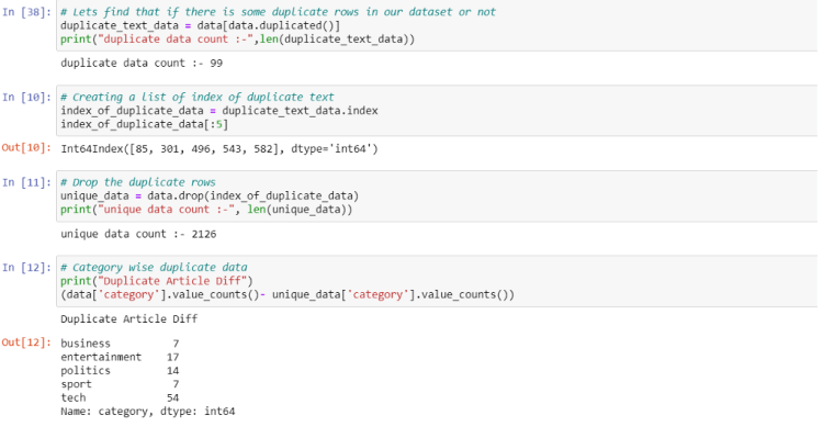
From the above code, we can see that this dataset also contains duplicate rows. We can first get the index of that duplicate data and after that, we can drop that rows from the real dataset using the drop() method. And also this dataset is already lowercased which is a necessary step in NLP problems. So we do not need to do it.

Vectorizing the Text

Now as we can see that the length of the dataset is around 2k which is not that much, so we should use ML algorithms because it works well with a small dataset.

But there is a problem that we can’t just feed text directly into the models we should convert this text and its categories into some kind of numbers which makes sense to our model.

Trending AI Articles:

1. How to automatically deskew (straighten) a text image using OpenCV

2. Explanation of YOLO V4 a one stage detector

3. 5 Best Artificial Intelligence Online Courses for Beginners in 2020

4. A Non Mathematical guide to the mathematics behind Machine Learning

For this, we will use tf–idf. For those people who are hearing this term first time. This helps to convert sentences into a big matrix of numbers like BOW(bag of words). And a special thing about this technique is that it helps to take care of words which occur frequently that cause model to become more biased towards it. And also helps to give significance to rare words that occur in very few documents.

For this, we will use the TfidfVectorizer function which can be imported from the sklearn library. As we know that, in a sentence, there are certain words like “is”, “and” etc. which make sense to humans but not much sense for computers, and especially if you doing a text classification task these words are worthless. These kinds of words are called stopwords and can be removed while creating tf-idf by setting stop_words = ‘english’.

Also making tf-idf vector by using only one word is not useful because in English we have many compound words(like ice cream), that make different meanings if we write them individually. And to capture such a group of words we use the concept of n-grams (like bi-grams making group of two words and tri-gram making group of three words.). So setting ngram_range=(1,3) means creating tf-idf matrix of 1(uni-grams), 2(bi-grams) and 3(tri-grams). And by setting min_df = 5 means ignoring the words which occur in less than 5 Document(news here) which helps to remove noise.

Factorize the Categories

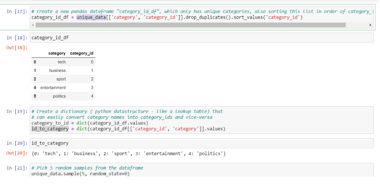
We have converted the text column to the matrix and now it’s time for the category column to converted into numbers, we can do this by factorize function. It assigns each unique category a unique integer value.

Also after prediction, we need to give output in form of text for that we are creating a dictionary that will map the factorized value back to its category text.

Decide the Model

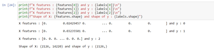
Now as we have everything ready to throw into ML models, it is time to initialize the model. But before that, we need to know what kind of problem is this is it regression or classification? So for that let’s take a look at our features and labels.

From the above figure, we can see that features are a matrix of size (2126, 14220) that means the number of sentences is 2126 and each sentence is transformed in tf-idf vector of size 14220 for each sentence, there is a corresponding value of labels which in reality is a category, and they are also encoded as a number. As we know that there are 5 categories and categories can’t be continuous value, we can frame this problem as a classification problem.

Initializing and fitting the Model

So we need to initialize the classification model for this. Let’s initialize 3 models at once so that we can choose the best of them according to accuracy.

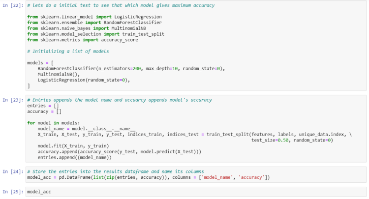
We will use RadomForest, Multinomial Naive Bayes, and Logistic Regression(actually logistic regression is a classification algorithm, don’t get confused by its name.)

Now we will iterate through these three models and observe the accuracy we achieved

We can see that Logistic Regression is doing well here and it achieved 97.27% accuracy. We can increase the accuracy of these models further by changing some parameters. But let leave this for now because we already achieved more than 95% accuracy.

Creating Logistic Regression Classifier

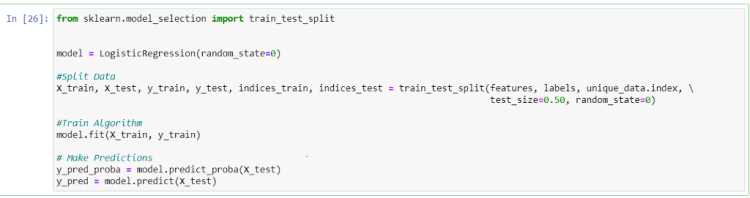
Now create the Logistic Regression model separately and let’s plot a confusion matrix plot too.

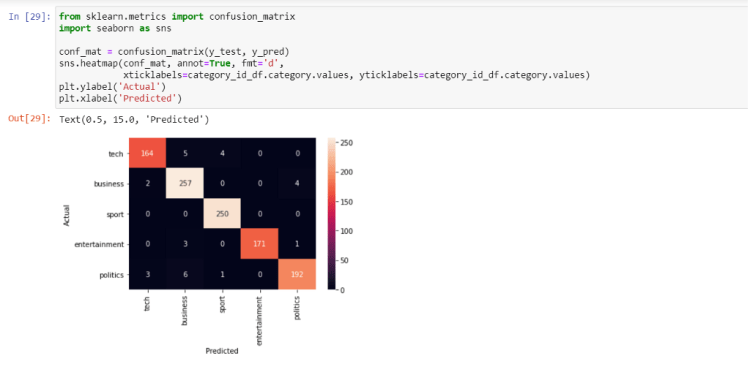
Quite a good performance isn’t it? Remember this, always try to go for the ML model first when you have a small dataset. If you try Deep learning on this dataset you will not reach this much accuracy in just a few steps.

Saving our Model

Now nearly everything is set. We just have to save our model

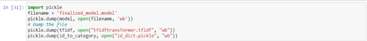
At last, we need to save our model, tf-idf transformer, and out id_to_category dictionary so that we can use this directly for our prediction in Web APP.

I know you may have got tired, so take a break for a few minutes and get ready to move into the next part ie.

Creating News Classification Django App (PART 1)

And wait wait wait ! before moving on further if you like this article then you can give me a clap 🙂 and I am thinking to create many articles on real Web deployment projects in the field of ML, CV, and Reinforcement learning. So if you do not want to miss them. Follow me and stay tuned 🙂

Readers are most welcome to notify me if something is mistyped or written wrong.

Github link for this project

My contacts.

Linked in

Github

Don’t forget to give us your ? !

Deploy your first ML model live on WEB (Part 1) was originally published in Becoming Human: Artificial Intelligence Magazine on Medium, where people are continuing the conversation by highlighting and responding to this story.

Via https://becominghuman.ai/deploy-your-first-ml-model-live-on-web-part-1-6939f353b6d9?source=rss—-5e5bef33608a—4

Cellular Automata Applications and Acceleration

For people with passing familiarity with the idea of cellular automata (CA), the first thing that comes to mind is probably John Horton Conway’s Game of Life. After Martin Gardner described Conway’s Game of Life (often abbreviated to Life, GOL, or similar) in his mathematical games column of Scientific American in 1970, the game developed into its own niche, attracting formal research and casual tinkering alike. With a significant population of dedicated hobbyists as well as researchers, it wasn’t long before people discovered and invented all sorts of dynamic machines implemented in the GOL. These can be quite complicated and include universal computers, some that can self-replicate. Other famous CA include Stephen Woflram’s Rule 110, proven to be Turing complete, capable of universal computation by Matthew Cook in 1998.

While Conway’s GOL is the most famous set of CA rules, the concept seems to have origins in conversations between John Von Neumann and Stanislaw Ulam in the 1940s when they both worked at Los Alamos National Laboratory. This eventually yielded a 29-state CA system which laid the foundations for Von Neumann’s universal constructor, a machine that operates in Neumann’s CA world and can make identical copies of itself.

What Are Cellular Automata?

Cellular automata can be generally described as a collection of cells, each with a state or states that change according to some rules based on each cell’s local context. Although cells are often arranged in rectangular 2D grids, the arrangement can be arbitrary, and while states are most often discrete, rules and states can also be continuously valued and even differentiable (more on that later). Many of the most interesting CA universes bear a striking resemblance to physical phenomena such as growth, diffusion, and flow, and CA have been described as the computer scientist’s discretized version of the physicist’s concept of fields. They are often used as the basis for physics models, and at least one prominent researcher thinks the resemblance is more than superficial.

Tiny Universes: Simulating Physics and Building Machines in Cellular Automata

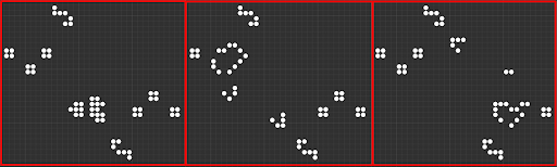
A glider generating pattern known as a Simkin glider gun. Here two “fish hooks,” stable patterns that destroy incident cells, consume the gliders before they travel to the edge of the grid. This example was simulated in Golly.

Trending AI Articles:

1. How to automatically deskew (straighten) a text image using OpenCV

2. Explanation of YOLO V4 a one stage detector

3. 5 Best Artificial Intelligence Online Courses for Beginners in 2020

4. A Non Mathematical guide to the mathematics behind Machine Learning

There has been significant research enthusiasm for CA beginning in the 1960s, and the field has seen steady growth in the number of papers published each year. They’ve been used to model everything from chemical reactions and diffusion, to turbulence, to epidemiology, and they are a cornerstone of fundamental complexity research. Given the visual similarity to a wide range of natural phenomena (remember, GOL rules were developed specifically to mimic life-like characteristics of growth and self-organization), it’s not surprising that CA have found so many applications in modeling and simulation. As mentioned above, cellular automata rules can often result in systems capable of universal computation, i.e. they can compute any algorithm that can be programmed. This holds true for the exceedingly simple 1D Rule 110 all the way up to the comparatively complicated 29-state Von Neumann system.

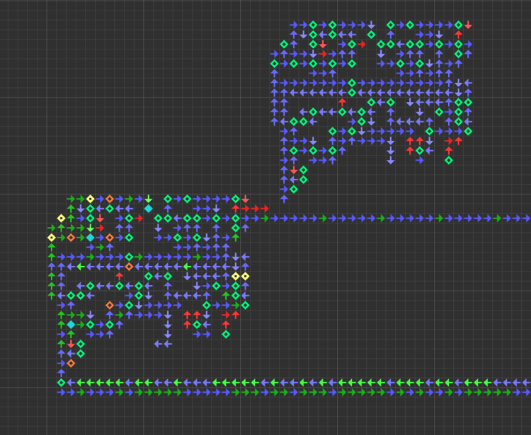
A small self-replicating constructor in Von Neumann’s CA universe. The constructor has built a copy of itself and is now copying the instruction sequence (the mostly blue line of arrows trailing off to the right) for the new machine. This example was simulated in Golly.

We’ve also seen both Turing complete computers and self-replicating universal constructors implemented in CA universes. Somewhat counterintuitively, Turing completeness is surprisingly easy to stumble upon by accident when building any system of sufficient complexity. However, we want to build not only computational systems but intelligent ones as well. We know they can compute, but can they learn?

Cellular Automata That Learn

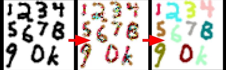
The interactive machine learning journal Distill.pub has a nascent research thread: “differentiable self-organizing systems.” They’ve only published two articles in this thread so far: a demonstration of self-generating and self-repairing graphical sprites, and self-classifying MNIST digits. Both articles are built around interactive visualizations and demonstrations with code, which is well worth a look for machine learning and cellular automata enthusiasts alike.

In the MNIST article, repeated application of CA rules eventually cause the cells to settle on a consensus classification (designated by color) for a given starting digit. Applying n updates to an image according to a set of CA rules is not altogether dissimilar to feeding that same image through an n-layer convolutional network, and so it is not surprising that one can use CA to solve a classic conv-net demo problem. In fact, as we’ll see later, CA rules can be implemented effectively as convolutions which means we can take advantage of the substantial development efforts in software, hardware, and systems for deep learning.

CA can do a lot more than “just” simulate physics, however the nature of CA computation doesn’t lend itself to conventional, serial computation on Von Neumann style architectures. To get good performance high-throughput parallelism is required. Luckily, while bespoke, single-purpose accelerators may offer some benefits, we don’t need to develop new accelerators from scratch. We can use many of the same software and hardware tools used to accelerate deep learning to get similar speedups with cellular automata universes.

Must Go Faster: Accelerating Cellular Automata

It’s useful to keep in mind that Von Neumann developed his 29-state CA using pen and paper, while Conway developed the 2-state GOL by playing with the stones and grid on a Go board. While it would probably be comparatively simple to use a computational search to discover new rules that satisfy the growth-like characteristics Conway was going for in Life, the simple tools used by Neumann and Conway in their work on cellular automata are a nice reminder that Moore’s law is not responsible for every inch of progress.

CA systems, like neural networks, are not particularly well-suited to implementation on typical general purpose computers. These tend to be based on the Von Neumann architecture (although multiple cores and cache memory do stretch the original concept), compute instructions sequentially, and emphasize low latency over parallelism. A cellular automaton universe, on the other hand, is inherently parallel and often massively so. Each individual cell must make identical computations based only on its local context.

The utility of CA systems led to several projects for dedicated CA processors, much like modern interest in deep learning has motivated the development of numerous neural coprocessors and dedicated accelerators. The specialized computers are sometimes called cellular automata machines (CAMs ). In the 1980s and 1990s CAMs were likely to be custom-designed for specific, often one-off purposes. The CAM-brain was an attempt to build a system using a Field Programmable Gate Array (FPGA) to evolve CA structures in order to simulate neurons and neural circuits. Systolic arrays, basically a mosaic of small processors that transform and transport data from and to one another, would seem to be an ideal substrate for implementing CA and indeed there have been several projects (including Google’s TPU) to take this approach. Systolic arrays sidestep one of the most often overlooked hurdles in high-performance computing, that of communications bottlenecks (the motivation behind Nvidia’s NVLink for multi-GPU systems and AMD’s Infinity Fabric.

Notable Projects for Building CA Acceleration Hardware

There have also been algorithmic speed-ups for the most popular CA rules: Hashlife, developed by Bill Gosper in the 1980s, uses memorization to speed up CA computations by remembering previously seen patterns. Just like special purpose accelerators for deep learning (e.g. Graphcore’s IPU or Cerebras’ massive wafer-scale accelerator), single-purpose accelerators for CA computations trade flexibility for speed.

Notable projects for building CA acceleration hardware include the cellular automata machine (CAM) by Norman Margolus and Tommasso Toffoli, which underwent several iterations in the 1980s. The first CAM prototype, described in 1984, could update a grid of 256 by 256 cells at a rate of 60 frames per second, in other words computing nearly 4 million updates a second. This was about a thousand times faster than execution on a comparable general purpose computer at the time. The speed-up was largely accomplished by mapping CA rules to memory and scanning over the grid rather than genuine parallelization. For comparison, the GPU PyTorch implementation in the next section updates more than 128 million cells each second on a personal workstation.

The supercomputer company Thinking Machines also devoted substantial efforts to building a massively parallel architecture for scientific computing. The so-called Connection Machine line of supercomputers were built with thousands of parallel processors arranged in a fashion akin to CA, but they were hardly the sort of computer one might purchase on a whim. The CA-based architecture made Connection Machines well-suited for many challenging scientific computing problems, but the company filed for bankruptcy in 1994.

Another project specifically for simulating neuronal circuits in CA (with the goal of efficiently controlling a robotic cat) was the CAM-brain project spearheaded by Hugo De Garis. The project went on for nearly a decade, building various prototype CA machines amenable to genetic programming and implemented in FPGAs, a sort of programmable hardware. While the project never got as far as their stated goal of controlling a robotic pet, they did develop a spiking neural model called CoDI and published a suite of preliminary experiments in 2001.

Hardware & Software Developments in Deep Learning

The examples mentioned so far have been pretty exotic. Not every researcher is ready to park a room-sized supercomputer in their office, and hard-wired solutions like application-specific integrated circuits (ASICs) are likely to be too static and inflexible for open-ended research. Luckily, as we’ve seen in the work on learning CA published in Distill, we can take advantage of the substantial hardware and software development efforts dedicated to deep learning. Luckily the deep learning tech stack is essentially interchangeable with research and development with cellular automata.

For flexible applications and exploratory development, CA implementations can take advantage of more general purpose GPUs and multicore CPUs for a significant speedup. We’ll investigate a simple demonstration of speeding up a CA system using the deep learning library PyTorch in the final section of this article.

Speeding up Life with PyTorch

In this simple benchmark we implement Conway’s Game of Life using convolution primitives in PyTorch. We’ll compare the PyTorch implementation on both GPU and CPU devices to a naïve loop-based implementation.

The PyTorch update function defaults to running a single step on the CPU, but these options can be specified by the user:

def gol_step(grid, n=1, device=”cpu”):

if torch.cuda.is_available():

device = device

else:

device = “cpu”

my_kernel = torch.tensor([[1,1,1], [1,0,1], [1,1,,1]])

my_kernel = my_kernel.unsqueeze(0).unsqueeze(0).float().to(device)

old_grid = grid.float().to(device)

while n > 0:

temp_grid = F.conv2d(old_grid, my_kernel, padding=1)#[:,:,1:-1,1:-1]

new_grid = torch.zeros_like(old_grid)

new_grid[temp_grid == 3] = 1

new_grid[old_grid*temp_grid == 2] = 1

old_grid = new_grid.clone()

n -= 1

return new_grid.to(“cpu”)

The naïve implementation scans through the grid using two loops, and it’s the sort of exercise you might implement as a simple “Hello World” when learning a new language. Unsurprisingly, it is very slow.

def gol_loop(grid, n=1):

old_grid = grid.squeeze().int()

dim_x, dim_y = old_grid.shape

my_kernel = torch.tensor([[1,1,1], [1,0,1], [1,1,1]]).int()

while n > 0:

new_grid = torch.zeros_like(old_grid)

temp_grid = torch.zeros_like(old_grid)

for xx in range(dim_x):

for yy in range(dim_y):

temp_sum = 0

y_stop = 3 if yy < (dim_y-1) else -1

x_stop = 3 if xx < (dim_x-1) else -1

temp_sum = torch.sum(my_kernel[\

1*(not(xx>0)):x_stop,\

1*(not(yy>0)):y_stop] \

* old_grid[\

max(0, xx-1):min(dim_x, xx+2),\

max(0, yy-1):min(dim_y, yy+2)])

temp_grid[xx,yy] = temp_sum

new_grid[temp_grid == 3] = 1

new_grid[old_grid*temp_grid == 2] = 1

old_grid = new_grid.clone()

n -= 1

return new_grid

A simple benchmark script iterates GOL updates ranging from 1 to 6000 steps, but you should feel free to write your own benchmarks script to compare the implementations on your own machine. Also note that I chose a grid size of 256 by 256 to match the 1984 CAM demo, but additional speedup is to be expected with larger grids.

import numpy as np

import time

import torch

import torch.nn as nn

import torch.nn.functional as F

for num_steps in [1, 6, 60, 600, 6000]:

grid = 1.0 * (torch.rand(1,1,64,64) > 0.50)

# naive implementation

if num_steps < 601:

t0 = time.time()

grid = gol_loop(grid, n=num_steps)

t1 = time.time()

print(“time for {} gol_loop steps = {:.2e}”.format(num_steps, t1-t0))

grid = 1.0 * (torch.rand(1,1,256,256) > 0.50)

# implementation with PyTorch (CPU)

t2 = time.time()

grid = gol_step(grid, n=num_steps)

t3 = time.time()

print(“time for {} gol steps = {:.2e}”.format(num_steps, t3-t2))

if num_steps < 601:

print(“loop/pt = {:.4e}”.format((t1-t0) / (t3-t2)))

grid = 1.0 * (torch.rand(1,1,256,256) > 0.50)

# implementation with PyTorch (GPU)

t4 = time.time()

grid = gol_step(grid, n=num_steps, device=”cuda”)

t5 = time.time()

print(“time for {} gol steps = {:.2e}”.format(num_steps, t5-t4))

if num_steps < 601:

print(“loop/pt = {:.4e}, loop/gpupt = {:.4e} pt/gpupt = {:.4e}”\

.format((t1-t0) / (t3-t2), (t1-t0) / (t5-t4), (t3-t2) / (t5-t4) ))

else:

print(“pt/gpupt = {:.4e}”.format((t3-t2) / (t5-t4) ))

Don’t forget to give us your ? !

Universes that Learn: Cellular Automata Applications and Acceleration was originally published in Becoming Human: Artificial Intelligence Magazine on Medium, where people are continuing the conversation by highlighting and responding to this story.

Via https://becominghuman.ai/universes-that-learn-cellular-automata-applications-and-acceleration-2ae4dae50296?source=rss—-5e5bef33608a—4

Vision Transformers — attention for vision task.

Recently there’s paper “An Image is Worth 16×16 Words: Transformers for Image Recognition at Scale” on open-review. It uses pretrained transformers at scale for vision tasks. Transformers are highly successful for language tasks, but haven’t seen that much success for vision. In vision, transformers are either applied in conjunction with Convolutional Neural Networks(CNN) or to replace some components of CNN. Recently transformers has shown good results on object detection (End-to-End Object Detection with Transformers). This paper applies transformers to vision task without using CNN and shows that state-of-art results can be obtained without CNN.

The Cost of attention is quadratic. So for images, every pixel needs to attend to every other pixel which is costly. There are different methods used to overcome this like local attention (attend to subset of input) or global attention. This paper uses global attention.

Architecture

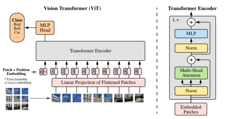
The architecture follows very closely the transformers. This is done to use transformer architecture that has scaled well for NLP tasks and optimised implementation of the architecture can be used out of box from different libraries. The difference came from how images are fed as sequence of patches to transformers.

Patch Embedding

Transformer receives 1D embedding as input. To handle 2D image input., the image is divided into sequence of flattened 2D fix size image patches. So , image of size H*W*C is divided into sequence of patches of size N*(P2*C), where P*P is size of patch.

Trending AI Articles:

1. How to automatically deskew (straighten) a text image using OpenCV

2. Explanation of YOLO V4 a one stage detector

3. 5 Best Artificial Intelligence Online Courses for Beginners in 2020

4. A Non Mathematical guide to the mathematics behind Machine Learning

Before passing the patches to transformer , Paper suggest them to put them through linear projection to get patch embedding. The official jax implementation uses conv layer for the same.(can be done by simple linear layer but its costly). Below is snippet of code from my pytorch implementation for the same.

As with BERT’s [class] token, learnable class token is concatenated to patch embedding, which serves as class representation.

To retain positional information of patches, positional embedding are added to patch embedding. Paper have explored 2D-aware variant as well as standard 1D embedding for position , but haven’t seen much advantage of one over the other.

Hybrid Architecture.

Alternative can be to use intermediate feature maps of a ResNet instead of image patches as input to transformers. The 2D feature map from earlier layers of resnet are flattened and projected to transformer dimension and fed to transformer. class token and positional embedding are added as mentioned.

Results

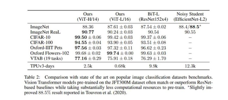
Vision transformer is pretrained on large datasets like Imagenet-1k, Imagenet-21k, JFT-300M. And based on task, it’s fine tuned on the task dataset. The table below shows the results of fine-tuning on vision transformer pretrained on JFT-300M.

You can find my repo for pytorch implementation here. I have used Imagenet-1k pretrained weights from https://github.com/rwightman/pytorch-image-models/ and updated checkpoint for my implementation. The checkpoint can be found here.

You can also find pytorch Kaggle Kernel for fine tuning vision transformer on tpu here.

References:

• https://openreview.net/forum?id=YicbFdNTTy
• https://github.com/google-research/vision_transformer
• https://github.com/rwightman/pytorch-image-models/

Don’t forget to give us your ? !

Vision Transformers — attention for vision task. was originally published in Becoming Human: Artificial Intelligence Magazine on Medium, where people are continuing the conversation by highlighting and responding to this story.

Via https://becominghuman.ai/vision-transformers-attention-for-vision-task-d0ef0fafe119?source=rss—-5e5bef33608a—4

Via https://becominghuman.ai/human-vs-machine-reinforcement-learning-in-the-context-of-snake-ae84d0b1f5d1?source=rss—-5e5bef33608a—4