How to evaluate the Machine Learning models? — Part 3
Congratulations everyone- who is reading this metric series, with this article we have came half way in the metric series. This is third part of the metric series where, we will discuss about predicting power score which act as substitute of the correlation and confusion metrics and derived from the confusion metrics which is very important when we evaluate the model using accuracy. The metric derived from the confusion metric act as a justification along with the confusion metric to justify our model. Below is the images of the metric which we are going to discuss in this article.
- Predicting Power score
Predictive power score is a normalized metric which has range [0,1], it shows up to what extend IV can be used to predict DV. It is alternative to correlation. It is very effective in following ways:
- It can detect and summaries linear and non-linear relationship also.
- It is asymmetric, i.e. IV to DV not vice versa.
It is slower to correlation in calculation but it is useful in many ways and can give accurate results. This article is focused on the confusion metric therefore I have not described in detail. For other correlation metrics article.
Jupyter Notebook: Link
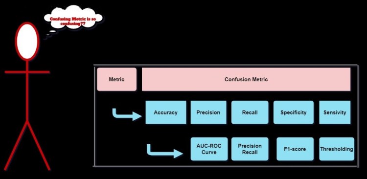
2. Confusion Metric
Confusion metric is like mother/father of classification metric from which many metric can be derived such as Accuracy, Precision and many other which we are going to discuss. It is applicable to machine learning as well as deep learning models.
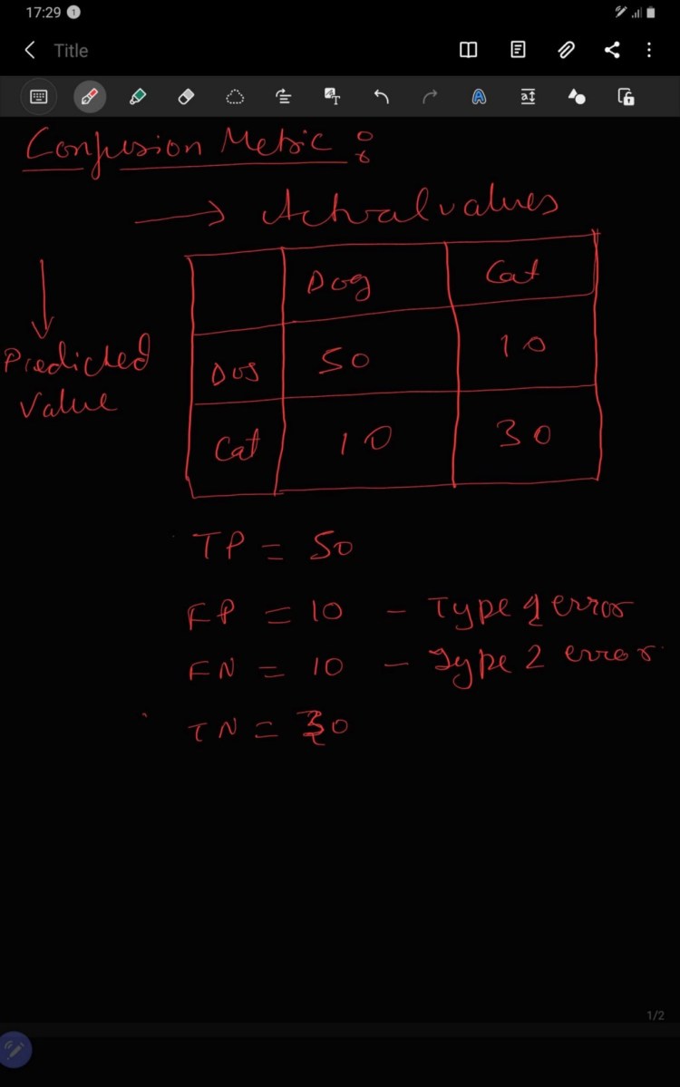
If confusion metric is a metric of size m *m ( m is no. of classes) , if we traverse row wise i.e. left to right it represent Actual Value and if we traverse column wise only it represent Predicted Value and the combination of the row can column give the count of the TP, TN, FP, and FN.

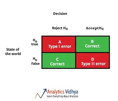
FN (False Negative) = Predicted value is Falsely predicted and the actual value is positive but the model predicted negative value . It is also known as Type 2 error.
FP (False Positive) = Predicted value is Falsely predicted and the actual value is negative but the model predicted positive value. It is also known as Type 1 error.
TN (True Negative) = Predicted value matches the actual value. The model predicted the negative value and the actual value is also negative.
TP (True Positive)= Predicted value matches the actual value. The model predicted the positive value and the actual value is also positive.

Why we need the Confusion metric?
Suppose we have dataset which has 90 dog images and 10 cat images and a model is trained to predict dog, where a trained model predicted 80 correct sample and 20 incorrect sample.
Jupyter Notebook: Link
2.1. Accuracy
Accuracy is defined as the no of correctly predicted sample( TN+ TP) to the total no. of samples (TN+TP+FN+FP).
Trending AI Articles:
1. How to automatically deskew (straighten) a text image using OpenCV
3. 5 Best Artificial Intelligence Online Courses for Beginners in 2020
4. A Non Mathematical guide to the mathematics behind Machine Learning
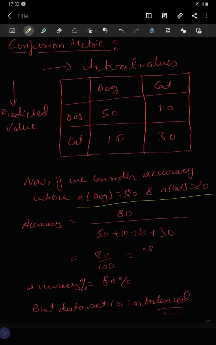
In above image, we can see accuracy is giving wrong data about the result i.e. model is saying it will predict dog 80% of the time, actually it is doing opposite. We saw that, the accuracy of the model is very good 80% but dataset is imbalance i.e. one class has more no of sample than other which makes model biased towards one class and hence in real world application it will not be able to work according to our expectation. So we need other metrics also which support our model more.
Jupyter Notebook: Link
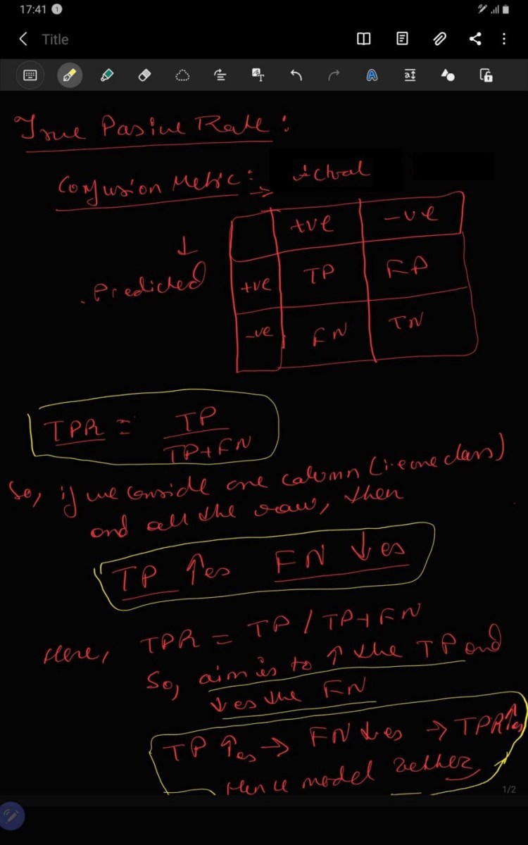
2.2. TPR
TPR is known as True Positive rate, which is ration of TP: ( TP+FN). Value of TPR is directly proportional to goodness of model i.e. TPR increases model becomes better. Alternative to accuracy metric.
Jupyter Notebook: Link
2.3. FNR
FNR is known as False Negative rate, which is ration of FN: ( TP+FN). Value of FNR is indirectly proportional to goodness of model i.e. FNR decreases model becomes better. Alternative to accuracy metric.

Jupyter Notebook: Link
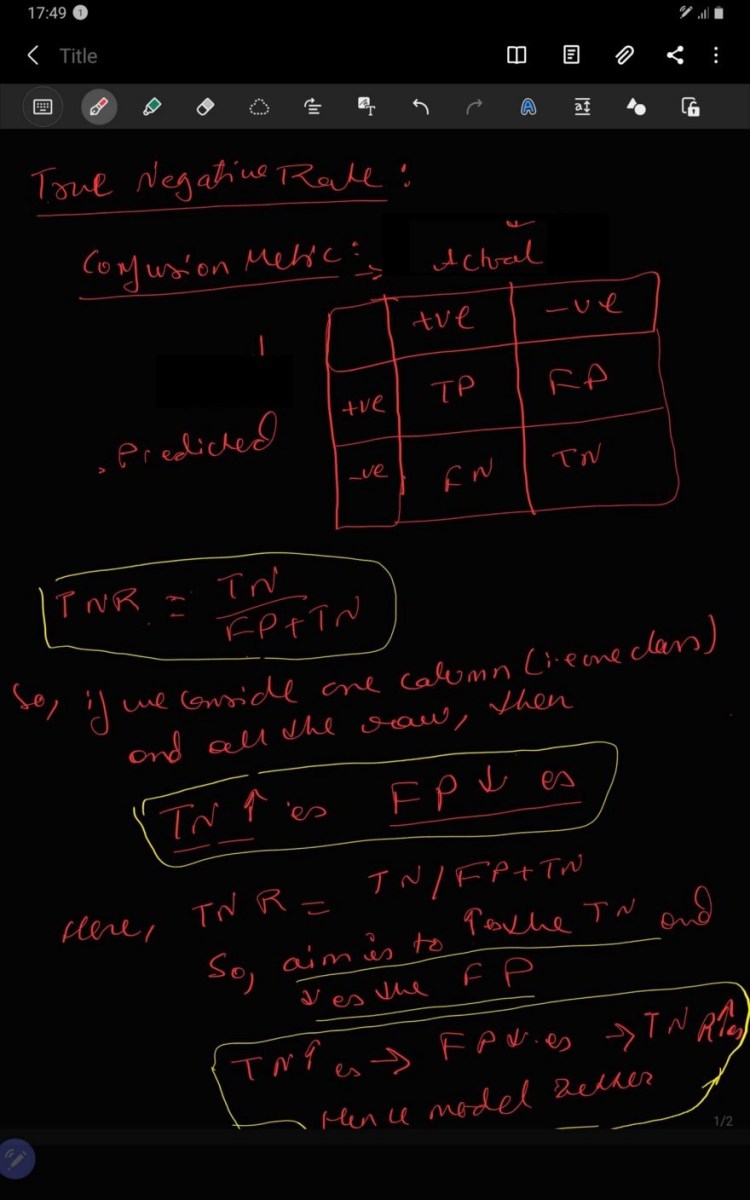
2.4. TNR
TNR is known as True Negative rate, which is ration of TN: ( FP+TN). Value of TNR is directly proportional to goodness of model i.e. FPR increases model becomes better. Alternative to accuracy metric.
Jupyter Notebook: Link
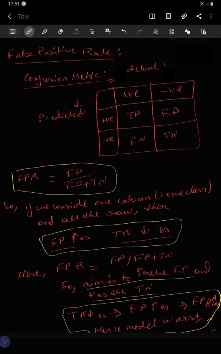
2.5. FPR
FPR is known as False Positive rate, which is ration of FP: ( FP+TN). Value of FNR is indirectly proportional to goodness of model i.e. FPR decreases model becomes better. Alternative to accuracy metric.
Jupyter Notebook: Link
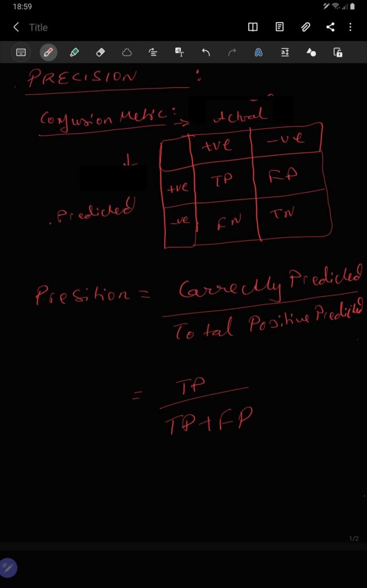
2.6. Precision
Precision tell us how many of the samples were predicted correctly to the all positive predicted samples i.e. TP:(TP+FP). We cannot afford to have more FP FP because it will degrade our model. It is very useful when FP is more important than the FN especially in terms of healthcare.
Jupyter Notebook: Link
2.7. Recall
Recall tell us how many of the samples were predicted correctly to the all the actual positive predicted samples i.e. TP:(TP+FN). We cannot afford to have more FN because it will degrade our model. It is very useful when FN is more important than the FP especially in terms of security of places.

High precision we will have low recall and vice versa. It is trade of between these two metric similar to Bias-Variance Tradeoff, so it depends upon the use case which metric we can select.

Jupyter Notebook: Link
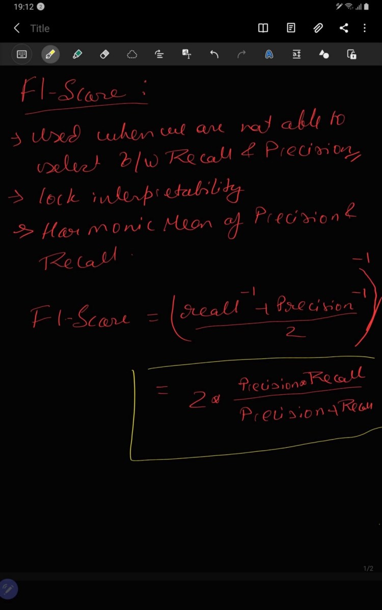
2.8. F1-score
As we have discussed above we precision and recall are inversely related and in some cases where we are unable to decide which metric to use so we procced with F1-score which is combination of precision and recall. F1-score is harmonic mean of precision and recall has high value when precision and recall are equal. It is always used with other evaluation metric because it lacks interpretation.
Jupyter Notebook: Link
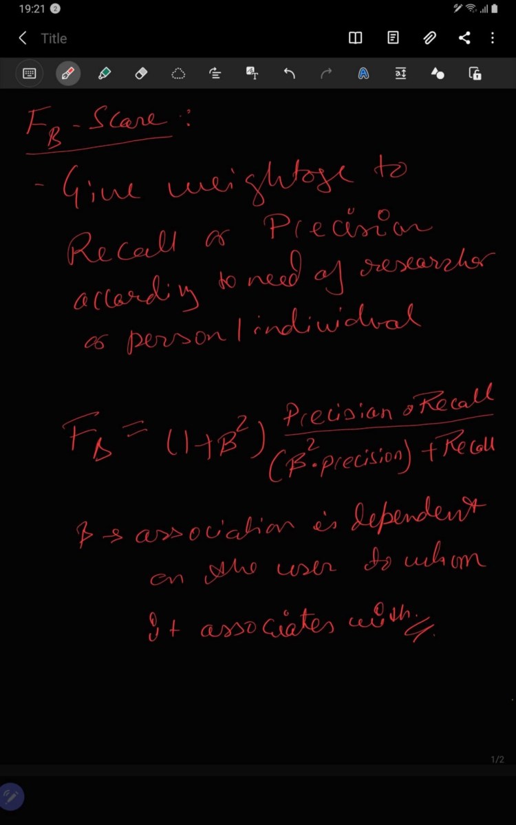
2.9. F-Beta Sore.
We have discussed earlier that F-score uses geometric mean instead of the arithmetic mean because Harmonic mean punishes penalize bigger value more.
If P=0 recall=1 then arithmetic mean=0.5, it is clear it is output of dumb model- ignore the input feature and predict one of the classes only. Now if we take Harmonic mean of Precision and recall, we will get 0. Some researchers can give more importance/ weight to precision or recall, so they can attach the adjustable parameter known as beta-square which will give beta times importance to precision or recall respectively.
Jupyter Notebook: Link
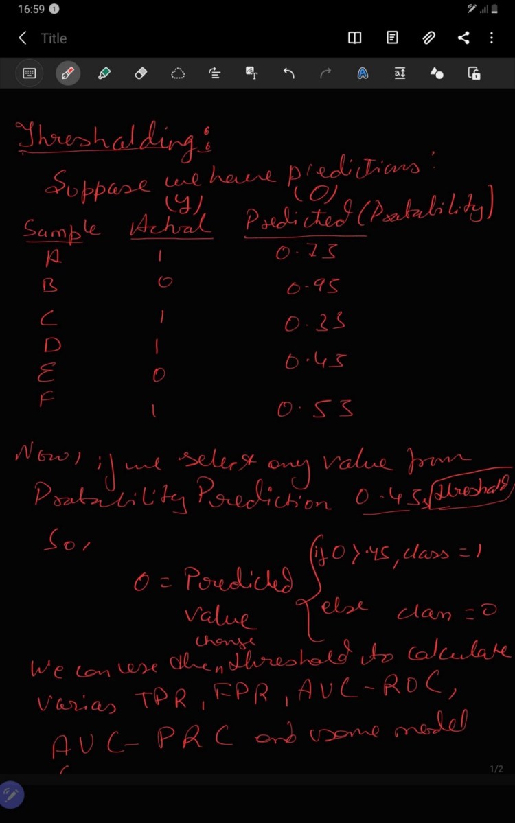
2.10. Thresholding
Thresholding is a technique in which is applied to the probability of the prediction of the models. Suppose you have used “softmax” as the activation layer in the output layer — gives probability of the prediction. In thresholding we can select a particular value so that if the predicted value is higher to the particular value we can classify into one class/label and if the predicted value is lower that the particular value we can classify into another class/label. This particular value is known as threshold and the process is called thresholding.
The threshold is determined by considering TP, TN, FP, and FN as well as the use case or business scenario.
Jupyter Notebook: Link
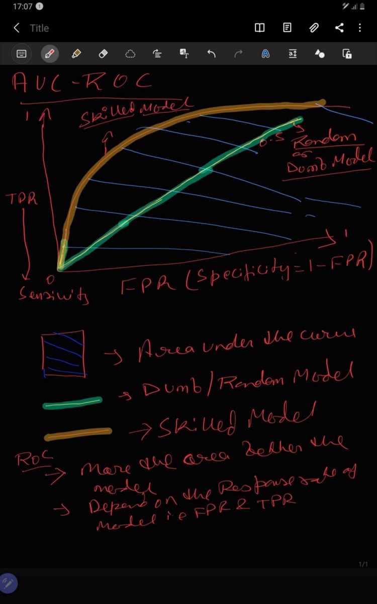
2.11. AUC — ROC
AUC is referred as Area Under the Curve i.e. the the amount of area which are under the line( linear or non linear). ROC means Receiver Operating Characteristic, initially it was used for differentiating noise from not noise but in recent years it is used very frequently in binary classification.
ROC gives trade-off between TP and FP where x- axis represent FPR and y-axis represent TPR. Total area of ROC is 1 unit because TPR and FPR value has range[0,1]. It can be clearly analyzed that more the area under the curve better the model as it can clearly differentiate between positive and negative class but AUC in ROC should be greater than 0.5 unit.
AUC = 1, then the binary classification model is able to perfectly differentiate between all the Positive and the Negative class points correctly.
AUC =0, then the classifier would be predicting all Negatives as Positives, and all Positives as Negatives.
0.5<AUC<1, there is a high chance that the binary classification model will be able to differentiate between the positive class values from the negative class values. This is so because the classifier is able to detect more numbers of True positives and True negatives than False negatives and False positives.
AUC=0.5, then the classifier is not able to distinguish between Positive and Negative class points. Meaning either the classifier is predicting random class for all the dataset.
Few more terms:
TPR is also known as Sensivity.
Specificity = 1- FPR
So, don’t get confused when you will see the combination of these words in any other blog/articles.
Steps to build AUC-ROC:
- Arrange the dataset on the basis on the predictions of probability in decreasing order.
- Set the threshold as the ith row of the prediction (for 1st take 1 prediction for second take 2nd as threshold).
- Calculate the value of TPR and FPR.
- Iterate through all the data point in dataset and repeat the step 1, 2 and 3.
- Plot the value of TPR (Sensivity) and FPR (Specificity = 1- FPR).
- Select the model with maximum AUC.
Jupyter Notebook: Link
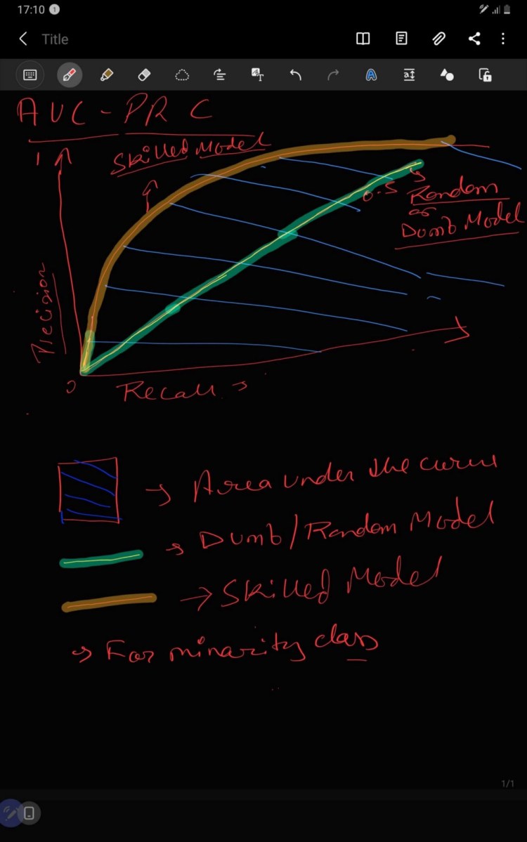
2.11. AUC — PRC
AUC is referred as Area Under the Curve i.e. the the amount of area which are under the line( linear or non linear). PRC means Precision Recall Curve, it is used very frequently in binary classification.
PRC gives trade-off between Precision and Recall where x- axis represent Precision and y-axis represent Recall. Total area of PRC is 1 unit because Precision and Recall value has range[0,1]. It can be clearly analyzed that more the area under the curve better the model as it can clearly differentiate between positive and negative class but AUC in PRC should be greater than 0.5 unit because of imbalance dataset as small change in prediction can show drastic change in AUC-PRC curve.
A binary classification model with correct predictions is depicted as a point at a coordinate of (1,1). A skillful model is represented by a curve that bows towards a coordinate of (1,1). A dumb binary classification model will be a horizontal line on the plot with a precision that is proportional to the number of positive examples in the dataset. For a balanced dataset this will be 0.5.The focus of the PR curve on the minority class makes it an effective diagnostic for imbalanced binary classification models. Precision and recall make it possible to assess the performance of a classifier on the minority class. Precision-recall curves (PR curves) are recommended for highly skewed domains where ROC curves may provide an excessively optimistic view of the performance
Steps to build AUC-PRC:
- Arrange the dataset on the basis on the predictions of probability in decreasing order.
- Set the threshold as the ith row of the prediction (for 1st take 1 prediction for second take 2nd as threshold).
- Calculate the value of Precision and Recall .
- Iterate through all the data point in dataset and repeat the step 1, 2 and 3.
- Plot the value of Precision and Recall.
- Select the model with maximum AUC.
Jupyter Notebook: Link
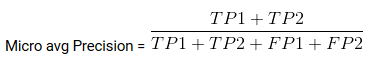
Micro average is the precision or recall of f1-score of classes.
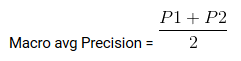
Macro average is the average of precision or recall of f1-score of classes.
Weighted average is just the weighted average of precision or recall of f1-score of classes.
Special Thanks:
As we say “Car is useless if it doesn’t have a good engine” similarly student is useless without proper guidance and motivation. I will like to thank my Guru as well as my Idol “Dr. P. Supraja”- guided me throughout the journey, from bottom of my heart. As a Guru, she has lighted the best available path for me, motivated me whenever I encountered failure or roadblock- without her support and motivation this was an impossible task for me.
Contact me:
If you have any query feel free to contact me on any of the below-mentioned options:
Website: www.rstiwari.com
Medium: https://tiwari11-rst.medium.com
Google Form: https://forms.gle/mhDYQKQJKtAKP78V7
Notebook for Reference:
Jovian Notebook: https://jovian.ai/tiwari12-rst/correlation
Jovian Notebook: https://jovian.ai/tiwari12-rst/metric-part3
References:
Environment Set-up: https://medium.com/@tiwari11.rst
YouTube : https://www.youtube.com/channel/UCFG5x-VHtutn3zQzWBkXyFQ
Don’t forget to give us your ? !


How to evaluate the Machine Learning models? — Part 3 was originally published in Becoming Human: Artificial Intelligence Magazine on Medium, where people are continuing the conversation by highlighting and responding to this story.