365 Data Science

Step by step guide to building a Deep Neural Network that classifies Images of Dogs and Cats.

Content Structure

Part 1:
1. Problem definition and Goals
2. Brief introduction to Concepts & Terminologies
3. Building a CNN Model
Part 2:
4. Training and Validation
5. Image Augmentation
6. Predicting Test images
7. Visualizing intermediate CNN layers

Problem Definition and Goals

Goal:
Build a Convolutional Neural Network that efficiently classifies images of Dogs and Cats.

Baseline Performance:
We have two classification categories — Dogs and Cats. So the probability for a random program to associate the correct category with the image is 50%. So, our baseline is 50%, which means that our model should perform well above this minimum threshold, else it is useless.

Dataset:
For this problem, we will use the Dogs vs Cats dataset from Kaggle, which has 25000 training images of dogs and cats combined.
You can download the dataset from here: Dogs vs. Cats

Brief Introduction to Concepts & Terminologies

Convolutional Neural Networks

Convolutional Neural Networks are a type of Deep Neural Networks. This NN uses Convolutions to extract meaningful information or patterns from the input features, which is further used to build the subsequent layers of neural network computations.

The following image is a visual example of how convolutions work

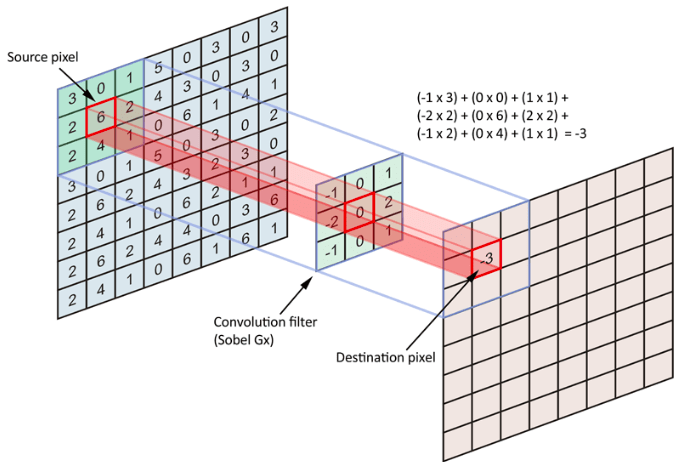
The left-most matrix is our input feature map.
The 3×3 matrix is our convolution filter.
The final matrix at the right is the output feature map.

The dimension of the convolution filter is usually called window size or kernel size of a convolution. This filter contains floating-point values, which can extract a certain pattern from the input feature map.

Trending AI Articles:

1. Fundamentals of AI, ML and Deep Learning for Product Managers

2. The Unfortunate Power of Deep Learning

3. Graph Neural Network for 3D Object Detection in a Point Cloud

4. Know the biggest Notable difference between AI vs. Machine Learning

The convolution window slides over every possible position on the input feature map and tries to extract patterns. As we see in the image, the convolution filter is nothing but a matrix that holds certain floating-point values. To apply the filter over the input feature map, we extract a patch from the input map with the exact dimension of the filter and perform matrix multiplication. When the same operation is performed over all possible patches in the input feature map, we compile them together as the output feature map.

Convolutional Neural Networks perform amazingly well on Image data and computer vision. Following are a few reasons, why CNN’s perform well on image data:

• One important difference between the Dense layer and the Convolutional layer is, dense layers are good at finding global patterns, while convolutional layers are good at finding local patterns.
• Convolutional layers also understand spatial data. Initial layers of the convnets (Convolutional Networks) detect low-level patterns like edges and lines, while the deeper layers detect more complex patterns like ears, nose, eyes, etc.
• Once learned, CNN can detect a pattern anywhere in the image. So, even if the images are sheared or modified, neural networks can still perform well.

Convnets: Shorthand representation of Convolutional Neural Networks

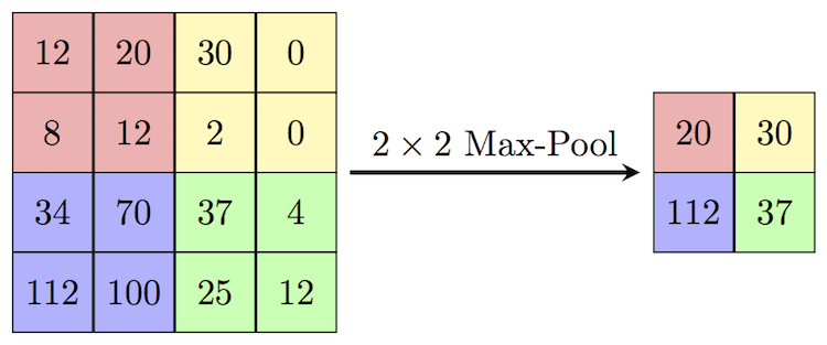
Max Pooling: Max pooling is a technique of aggressive downsampling of the feature map.

This is a 2×2 Max Pooling example. A 2×2 window slides over the feature map, and extracts only the maximum value from the window frame, and creates a new downsampled feature map. 2×2 MaxPooling with a stride of 2, downsamples the image by half. When 2×2 MaxPooling is applied over the 4×4 matrix, the result will be a 2×2 matrix.

Note: MaxPooling is preferred more over AveragePooling, because, it is more useful to have max value information of a pixel rather than to have the mean value of the values in the window.

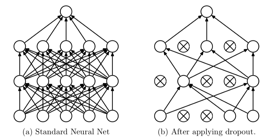
Dropout: Dropout is a popular technique in deep learning, where we ask the system to randomly ignore features in the neural network. This approach is used to prevent the neural network from overfitting and make sure it doesn’t learn some non-important patterns in the input data.

Batch Normalization: Batch Normalization speeds up the training process and helps the model learn from the training data. I highly suggest you look up this video Batch Normalization — EXPLAINED! by CodeEmporium YouTube channel.

For this particular model, we will make use of all these components explained above to build the Convolutional Neural Network to detect cats and dogs.

Building a CNN Model

A Typical CNN:
The following image is a descriptive representation of how a convolutional neural network will look like.

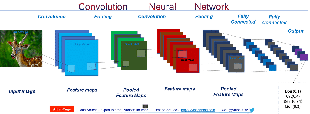
The input image is fed to the neural network. The Convnet then performs convolutions over the input image. Each convolution filter will result in its own output feature map. As we can look at the image, multiple convolutional filters are applied over the input image, as a result, we have transformed a single image into multiple output feature maps(Check the blue blocks).

Each feature map will hold specific information about the image. The number of these layers is called the depth of the channels.

Next, comes the pooling stage. In pooling, we downsize the input feature map, while retaining the most useful information. So, each value in the feature map after max-pooling will represent a larger patch of the input feature map. Max pooling helps convnets to detect more complex patterns with less computing power.

Multiple convolutional layers and max-pooling layers can be arranged successively to form the deep neural network. The number of layers and the depth of each convolutional layer are provided by us, there are no strict guidelines for these hyperparameters and we can experiment on our own to find the combination that works best for our model.

Finally, these convolutional layers are connected to a Dense layer(Fully connected), or a regular neural network. We are free to add multiple layers in this dense layer as well. The final output layer of this neural network will have two nodes, one for each class (Dogs vs Cats). There is another way to approach where we only go for a single output neuron (That outputs the binary value, Is it a cat? yes/no).

Enough of theory, let’s get practical:

Step 1: Creating a Sequential Model. Sequential models indicate that the layers of the neural network are stacked one after another. Convnets use Sequential architecture.

We will make use of the Keras library to build the Convolutional neural network. We will first create a sequential model first, and layers one by one to the network.

from keras import models, layers

# Create a Sequential model
model = models.Sequential()

Step 2: Add a Convolution Layer

IMAGE_SHAPE = (150, 150, 3)

# Create a Conv2D Layer
model.add(layers.Conv2D( filters = 32, 
                         kernel_size = (3, 3), 
                         activation='relu', 
                         input_shape=IMAGE_SHAPE) )

The 2D Convolutional layer is available in the Keras library under the ‘layers’ module. A convolutional layer requires a number of filters, kernel size, and activation hyperparameters to create the object. Additionally, for the first layer of the model, we pass the dimension of the input image as well.

filters: Number of Convolution filters the conv2d layer should create
kernel_size: window size of the convolutional filter
activation: which activation function should the layer use
input_shape: the dimension of the input feature map

For further layers of this network, we need not explicitly provide the dimensions of the input feature map, Keras will calculate the dimensions on its own.

After this step, we have a neural network with a single convolutional layer that creates an output feature map with a depth of 32.

Step 3: Add a BatchNormalization Layer and Dropout layer

The next step is to add Batch Normalization to our neural network. BatchNormalization and Dropout layers are also defined under the Keras.layers module, so we can make use of the library to quickly add the layers to our model.

# Add Batch Normalization layer
model.add(layers.BatchNormalization())

# Add drop out layer with 25% dropout rate
model.add(layers.Dropout(0.25))

BatchNormalization does take input hyperparameters, but for our current problem, it’s not required. If you are interested, you can take a look at the official documentation: BatchNormalization

For the Dropout layer, we pass one parameter, a floating-point value that represents the dropout rate. In the above example, 0.25 represents 25%, so 25% of the output features will be randomly ignored in further computations.

Step 4: Downsizing using MaxPooling

The next step is to create a MaxPooling layer with a 2×2 kernel, which downsamples the input image by half. This helps convolution layers understand more complex patterns.

model.add(layers.MaxPooling2D(pool_size=(2, 2))) 

Step 5: Build a deep network

Add more convolution layers(Step 2) to the model, in combination with other layers like MaxPooling2d(Step 4), Dropout, and BatchNormalization(Step 3) to build a deep neural network. You can experiment with the hyperparameters too.

Deeper the network, the deeper the understanding of the data. But a deeper network also means more time for training and requires more computing power. It’s enough to build a model that is borderline complex enough to perform well on the dataset, but not too complex. Extremely complex deep networks might be overkill for the problem at hand.

Here is an example of a deep convolutional network that you can refer

    model = models.Sequential()
    
    model.add(layers.Conv2D(32, (3, 3), activation='relu', input_shape=IMAGE_SHAPE))
    model.add(layers.BatchNormalization())
    model.add(layers.MaxPooling2D(pool_size=(2, 2)))
    model.add(layers.Dropout(0.20))
    
    model.add(layers.Conv2D(64, (3, 3), activation='relu'))
    model.add(layers.Conv2D(64, (3, 3), activation='relu'))
    model.add(layers.BatchNormalization())
    model.add(layers.MaxPooling2D(pool_size=(2, 2)))
    model.add(layers.Dropout(0.25))
    
    model.add(layers.Conv2D(128, (3, 3), activation='relu'))
    model.add(layers.Conv2D(128, (3, 3), activation='relu'))
    model.add(layers.Conv2D(128, (3, 3), activation='relu'))
    model.add(layers.BatchNormalization())
    model.add(layers.MaxPooling2D(pool_size=(2, 2)))
    model.add(layers.Dropout(0.30))
    
    model.add(layers.Conv2D(256, (3, 3), activation='relu'))
    model.add(layers.BatchNormalization())
    model.add(layers.MaxPooling2D(pool_size=(2, 2)))

Step 6: Add Dense Layers and Output layers

So far the network architecture that we have built is well suited for extracting the patterns from the feature map, but we don’t have a prediction system that helps us classify the input as either dog or a cat. In order to perform the task, we can feed the patterns detected by the convolutional neural network to another dense neural network, which can then classify the images as dogs or cats.

The dense neural networks take 1D tensors as input, while the final output from the convolutional network is a 3D tensor. So we perform the Flatten operation to convert the 3D tensor into a one-dimensional tensor that can be provided as input to the dense/fully connected neural network.

# Flatten the convolutional layer output
model.add(layers.Flatten())

# Create a dense layer with 512 hidden units
model.add(layers.Dense(512, activation='relu'))

# Output layer - 2 Units(Dogs, Cats)
model.add(layers.Dense(2, activation='softmax'))

Dense layer hyperparameters:
units: the first parameter, which takes the number of hidden units in this particular layer.
activation: activation function that the neurons of this layer should use.

The final output layer of this dense layer contains two neurons, one for dog and the other for the cat. Using SoftMax activation outputs a probabilistic value for each category.

For example, let’s assume the first neuron outputs the probability of the image being a dog, and the second neuron outputs the probability of the image is a cat. if we give an image to the model, and the model produces output values [0.89, 0.11], it means that the probability of the image being a dog is 89%.

Step 7: Compiling the model

We have now defined the architecture of our convolutional neural network model. Next step is to compile the model so that we can start training the model.

Compiling the model requires three inputs, the optimizing method, loss function, and the metrics.

Loss function (loss): This is the function that our model will try to reduce during the training process.
Optimizing method (optimizer): This indicates the method we are asking the model to use, to reduce the loss function.
Metrics(metrics): We will evaluate the performance of our model using the metrics provided here.

# Compiling the model
model.compile(loss='categorical_crossentropy', optimizer='rmsprop', metrics=['accuracy'])

categorical_crossentropy is a loss function that is used for multiclass classification problems. Here we have two classes(Dogs and Cats), so we use this as the loss function to train the model.

rmsprop — This is a popular optimizing method, we can experiment with different optimizers such as adam optimizer, adagrad optimizer. But to keep things simple, I have used rmsprop here, and also rmsprop works well for almost all the classification problems.

The remaining sections Training and Validation, Image Augmentation, Predicting the test dataset will be covered in the next blog post.

100MLProjects
This project is done as a part of #100MLProjects, a challenge that I set myself to master Machine Learning and Deep Learning concepts by doing 100 Projects. All the projects are available in my GitHub repository — #100MLProjects.

If you like this project, comment below, star the GitHub project repo.
If you are an expert, I would like to hear your comments and advise, I’m available at WriteTo@Laxmena.com. Also, I’ve attached the URL to my LinkedIn below.

Have a great day, Happy coding!

• Lakshmanan Meiyappan – Chennai, Tamil Nadu, India | Professional Profile | LinkedIn
• laxmena – Overview

Don’t forget to give us your ? !

Beginners Guide -CNN Image Classifier | Part 1 was originally published in Becoming Human: Artificial Intelligence Magazine on Medium, where people are continuing the conversation by highlighting and responding to this story.

Via https://becominghuman.ai/beginners-guide-cnn-image-classifier-part-1-140c8a1f3c12?source=rss—-5e5bef33608a—4