365 Data Science

Computer Goes Brrr: Revisiting Sutton’s Bitter Lesson for Artificial Intelligence

A Look Back at Richard Sutton’s Bitter Lesson in AI

Not that long ago, in a world not far changed from the one we inhabit today, an ambitious project at Dartmouth College aimed to bridge the gap between human and machine intelligence. That was 1956, and while the Dartmouth Summer Research Project on Artificial Intelligence wasn’t the first project to consider the potential of thinking machines, it did give it a name and inaugurated a pantheon of influential researchers. In the proposal put together by John McCarthy, Marvin Minsky, Claude Shannon, and Nathaniel Rochester, the authors lay out ambitions that seem quaint today in their naïve ambition:

“An attempt will be made to find how to make machines use language, form abstractions and concepts, solve kinds of problems now reserved for humans, and improve themselves. We think that a significant advance can be made in one or more of these problems if a carefully selected group of scientists work on it together for a summer.” –A Proposal for the Dartmouth Summer Research Project on Artificial Intelligence, 1955

Artificial Intelligence At The Beginning

In the intervening period between then and now, there have been a series of waxing and waning periods of enthusiasm for AI research. Popular approaches in 1956 included cellular automata, cybernetics, and information theory, and throughout the years there would be debuts and revivals with expert systems, formal reasoning, connectionism and other methods all taking their turn in the limelight.

The current resurgence of AI is being driven by the latest incarnation of the connectionism lineage in the form of deep learning. Although a few new ideas have made major impacts in the field, (attention, residual connections, and batch normalization to name a few), most of the ideas about how to build and train deep neural networks had already been proposed in the 80s and 90s. And yet the role of AI or AI-adjacent technology today certainly isn’t what a researcher active in one of the previous “AI springs” would have envisaged. Few could have predicted the prevalence and societal repercussions of adtech and algorithmic newsfeeds, for example, and I’m sure many would be disappointed at the lack of androids in present day society.

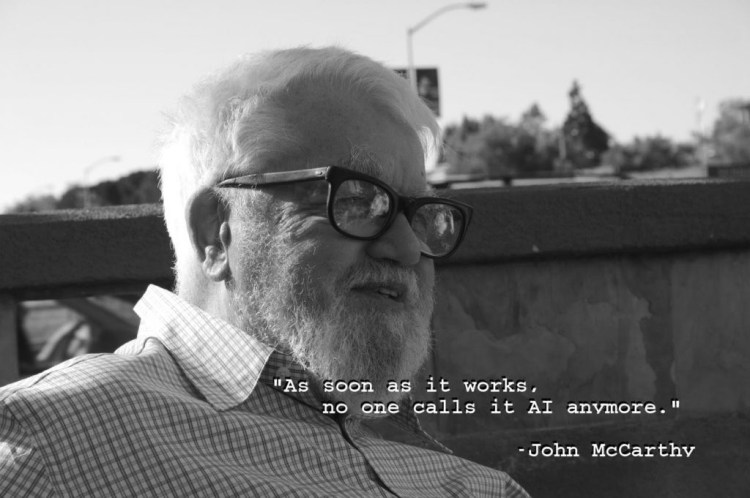
John McCarthy, co-author of the Dartmouth proposal and coiner of the term Artificial Intelligence. Image CC BY SA flickr user null0.

A quote attributed to John McCarthy complains AI techniques that find real-world use invariably become less impressive, and lose the “AI” moniker in the process. That’s not what we see today, however, and perhaps we can blame venture capital and government funding bodies for incentivizing the opposite. A survey by London venture capital firm MMC found that up to 40% of self-described AI startups in Europe didn’t actually use AI as a core component of their business in 2019.

The Difference Between Deep Learning and AI Research

The difference between the deep learning era and previous highs in the AI research cycles seems to come down to our place on the sigmoidal curve of Moore’s Law. Many point to the “ImageNet Moment” as the beginning of the current AI/ML resurgence, when a model known as AlexNet won the 2012 ImageNet Large Scale Visual Recognition Competition (ILSVRC) by a substantial margin. The AlexNet architecture wasn’t much different from LeNet-5 developed more than two decades earlier.

AlexNet is slightly larger with 5 convolutional layers to LeNet’s 3, and 8 total layers vs 7 for LeNet (although those 7 layers include 2 pooling layers). The big breakthrough, then, came from implementing neural network primitives (convolutions and matrix multiplies) to take advantage of parallel execution on graphics processing units (GPUs), and the size and quality of the ImageNet dataset developed by Fei-Fei Li and her lab at Stanford.

Trending AI Articles:

1. Fundamentals of AI, ML and Deep Learning for Product Managers

2. The Unfortunate Power of Deep Learning

3. Graph Neural Network for 3D Object Detection in a Point Cloud

4. Know the biggest Notable difference between AI vs. Machine Learning

Interested in an AI workstation?
Learn more about Exxact deep learning workstations starting at $3,700

The Bitter Lesson in Hardware Acceleration

Hardware acceleration is something that today’s deep learning practitioners take for granted. It’s part and parcel to popular deep learning libraries like PyTorch, TensorFlow, and JAX. The growing community of deep learners and commercial demand for AI/ML data products fuels a synergistic feedback loop, that fuels good hardware support. As new hardware accelerators based on FPGAs, ASICs, or even photonic or quantum chips, become available, software support in the major libraries is sure to follow close behind.

The impact of ML hardware accelerators and more available compute on AI research was succinctly described in a short and (in)famous essay by Richard Sutton called “The Bitter Lesson.” In the essay Sutton, who literally (co)-wrote the book on reinforcement learning, appears to claim that all the diligent efforts and clever hacks that AI researchers strive to make amount to very little in the grand scheme of things. The main driver of AI progress, according to Sutton, is the increasing availability of compute applied to simple learning and search algorithms we already have, with a minimum of hard-coded human knowledge. Specifically, Sutton argues for AI based only on methods that are as general as possible, such as unconstrained search and learning.

It’s no surprise that many researchers had contrary reactions to Sutton’s lesson. After all, many of these people have dedicated their lives to developing clever tricks and theoretical foundations to move the needle on AI progress. Many researchers in AI are not just interested in figuring out how to best state-of-the-art metrics, but to learn something about the nature of intelligence in general and, more abstractly, the role of humanity in the universe. Sutton’s statement seems to support the unsatisfying conclusion that searching for insights from theoretical neuroscience, mathematics, cognitive psychology, etc., are useless for driving AI progress.

Meme from gwern.net. Here’s another one.

Saccharine Skeptics of the Bitter Lesson

Noteworthy criticisms of Sutton’s essay include roboticist Rodney Brooks’ “A Better Lesson,” a tweet sequence from Oxford computer science professor Shimon Whiteson, and a blog post by Shopify data scientist Katherine Bailey. Bailey argues that, while Sutton may be right for the limited-scope tasks that serve as metrics for the modern AI field, that short-sightedness is missing the point entirely. The point of AI research is ultimately to understand intelligence in a useful way, not to train from scratch a new model for every narrow metric-based task, incurring substantial financial and energy costs along the way. Bailey thinks that modern machine learning practitioners too often mistake the metric for the goal; researchers did not set out to build superhuman chess engines or Go players for their own sake, but because these tasks seem to exemplify some aspect of human intelligence in a crucial way.

Brooks and Whiteson argue that in fact, all the examples used by Sutton as free from human priors are in fact the fruit of substantial human ingenuity. It’s hard to imagine deep neural networks that perform as well as modern ResNets without the translational invariance of convolutional layers, for example. We can also identify specific areas where current networks fall short, a lack of rotational invariance or color constancy are just 2 examples out of many. Architectures and training specifics also tend to make heavy use of human intuition and ingenuity. Even if neural architecture search (NAS) automation can sometimes find better architectures than models designed manually by human engineers, the component space available to NAS algorithms is vastly reduced from the space of all possible operations, and this narrowing down of what’s useful is invariably the purview of human designers.

Whiteson argues that complexity necessitates, rather than obviates, human ingenuity in building machine learning systems.

There is substantial overlap between vocal critics of the bitter lesson and researchers that are skeptical of deep learning in general. Deep learning continues to impress with scale, despite ballooning compute budgets and growing environmental concerns about energy usage. And there’s no guarantee that deep learning won’t run up against a wall at some point in the future, possibly quite soon.

When will marginal gains no longer justify the additional expense? One reason that progress in deep learning is so surprising is that the models themselves can be nigh inscrutable; the performance of a model is an emergent product of a complex system with millions to billions of parameters. It’s difficult to predict or analyze what they may ultimately be capable of.

Perhaps we should all take to heart a lesson from the quintessential reference on good old-fashioned AI (GOFAI): “Artificial Intelligence: A Modern Approach” by Stuart Russell and Peter Norvig. Nestled towards the end of the last chapter we find this warning that our preferred approach to AI, in our case deep learning, may be like:

“… trying to get to the moon by climbing a tree; one can report steady progress, all the way to the top of the tree.“ -AIMA, Russel and Norvig

The authors are paraphrasing an analogy from a 1992 book by Hubert Drefyfus “What Computers Can’t Do,” which frequently returns to the analogy of the arboreal strategy for lunar travel. While many a primitive Homo sapiens may have attempted this method, actually reaching the moon requires one to come down from the trees and get started on building the foundations of a space program.

The Results Speak for Themselves

As appealing as these criticisms are, they can come across as little more than sour grapes. While academics are put off by the intellectually unfulfilling cry for “more compute,” researchers at large private research institutions continue to make headlines from projects where engineering efforts are primarily applied directly to scaling.

Perhaps most notorious for this approach is OpenAI.

Key personnel at OpenAI, which transitioned from a non-profit to a limited partnership corporate structure last year, have never been shy about their predilection for massive amounts of compute. Founders Greg Brockman and Ilya Sutskever fall firmly within Richard Sutton’s Bitter Lesson camp, as do many of the technical staff at the growing company. This has led to impressive feats of infrastructural engineering to empower the big training runs OpenAI turns to for reaching milestones.

OpenAI Five was able to beat the (human) Dota 2 world champions, Team OG, and it only took the agents 45,0000 simulated years, or about 250 years of gameplay per day to learn to play. That comes out to 800 petaflop/s-days over 10 months. Assuming a world-leading efficiency of 17 Gigaflop/s per watt, that comes to over 1.1 gigawatt hours: about 92 years of electricity use for an average US home.

Another high-profile and high-resource project from OpenAI was their Dactyl dexterity project with the Shadow robotic hand. That project culminated in achieving dexterous manipulation sufficient to solve a Rubik’s cube (although a deterministic solver was used to choose moves). The Rubik’s cube project was built on approximately 13,000 years of simulated experience. Comparable projects from DeepMind, such as AlphaStar (44 days of 384 TPUs training 12 agents, had thousands of years of simulated gameplay) or the AlphaGo lineage (AlphaGo Zero: ~1800 petaflop/s days) also required massive expenditures of computational resources.

But They Don’t Always Agree

A remarkable exception from the trends noted in The Bitter Lesson can be seen in the AlphaGo family of game playing agents, which actually required less compute as they reached better performance. The AlphaGo lineage is indeed a curious case that doesn’t fit kindly into the bitter lesson framework. Yes, the project started off with a heavy dose of overpowered HPC training, AlphaGo ran on 176 GPUs and consumed 40,000 watts at test time. But each successive iteration of AlphaGo up to MuZero used less energy and compute for both training and play.

In fact, when AlphaGo Zero played against StockFish, the pre-deep learning state-of-the-art chess engine, it used substantially less, and more specialized, search than StockFish. Whereas AlphaGo Zero did use Monte Carlo tree search, it was guided by a deep neural network value function. The alpha-beta pruning search employed by Stockfish is more general, and Stockfish evaluated about 400 times as many board positions as AlphaGo Zero during each turn.

Should Bitter Lesson Outperform More Specialized Methods?

You’ll recall that unrestrained search was a principal example of a general method used by Sutton, and if we take the Bitter Lesson at face value, it should outperform a more specialized method that performs narrowed search. Instead what we saw with the AlphaGo lineage was that each successive iteration (AlphaGo, AlphaGo Zero, AlphaZero, and MuZero) was more generally capable than the last, but employed more specialized learning and search. MuZero replaced the ground truth game simulator used for search by all its Alpha predecessors with a learned deep model for game state representation, game dynamics, and prediction.

Designing the learned game model represents substantially more human development than the original AlphaGo, while MuZero expanded in terms of general learning ability by reaching SOTA performance on the 57 game Atari benchmark, in addition to chess, shogi and Go learned by previous Alpha models. MuZero used 20% less computation per search node than AlphaZero, and, in part thanks to hardware improvements, 4 to 5 times fewer TPUs during training.

Stockfish, salted and hanging out to dry (after being defeated by AlphaGo Zero). Public Domain image.

The AlphaGo lineage of machine game players from Deepmind are a particularly elegant example of progress in deep reinforcement learning. If the AlphaGo team managed to continuously build capability and general learning competence while decreasing computational requirements, doesn’t that directly contradict the bitter lesson?

If so, what does it tell about the quest for general intelligence? RL is, according to many, a good candidate for building artificial general intelligence due to the similarity to how humans and animals learn in response to rewards. There are other modes of intelligence that some preferred as candidates for AGI precursors, however.

Language Models: The Sultans of Scale

One reason Sutton’s article is getting a fresh round of attention (it was even recently reposted as a top article on KDNuggets) is the attention-grabbing release of OpenAI’s GPT-3 language model and API. GPT-3 is a 175 billion parameter transformer, eclipsing the previous record for language model size held by Microsoft’s Turing-NLG, by a little more than 10 times. GPT-3 is also more than 100 times larger than the “too dangerous to release” GPT-2.

The release of GPT-3 was a central part of the announcement of OpenAI’s API beta. Basically, the API gives experimenters access to the GPT-3 model (but not the ability to fine-tune parameters) and control over several hyperparameters that can be used to control inference. Understandingly, the beta testers lucky enough to get access to the API approached GPT-3 with much enthusiasm, and the results were impressive. Experimenters built text-based games, user interface generators, fake blogs, and many other creative uses of the massive model. GPT-3 is markedly better than GPT-2, and the only major difference is scale.

The trend toward larger language models predates the big GPTs, and isn’t limited to research at OpenAI. But the trend has really taken off since the introduction of the first transformer in “Attention is all You Need”. Transformers have been steadily creeping into the tens of billions of parameters, and it wouldn’t surprise me if there was a trillion parameter transformer demonstrated in about a year or so. Transformers seem to be particularly amenable to improving with scale, and the transformer architecture is not limited to natural language processing with text. Transformers have been adapted for reinforcement learning, predicting chemical reactions, generating music, and generating images. For a visual explainer of the attention mechanism used by transformer models, read this.

At the current rate of model growth someone will train a model with a comparable number of parameters as the total synapses in a human brain (~100 trillion) within a few years. Science fiction is riddled with examples of machines reaching consciousness and general intelligence simply by accruing sufficient scale and complexity. Is that the end result we can expect from growing transformers?

The Answer to the Future of AI Lies Between Extremes

The performance of big transformers is certainly impressive, and continued progress due to scale seems to be in line with the Bitter Lesson. Triaging all other AI efforts behind scale remains inelegant and unsatisfying, however, and the concomitant demand for energy resources yields its own concerns. Training in the cloud separates many researchers at big labs from the physical reminders of training inefficiency. But anyone who runs deep learning experiments in a small office or apartment has a constant reminder in the stream of hot air constantly exiting the back of their workstation.

Portrait of Richard Sutton modified CC BY Steve Jurvetson

The carbon output of training a large NLP transformer with hyperparameter and architecture search can easily be larger than the combined carbon contributions of all other activities for individuals on a small research team.

We know that intelligence can run on hardware that runs continuously on about 20 watts (plus another ~80 watts for supporting machinery), and if you doubt that you should verify the existence proof between your ears. In contrast, the energy requirements used to train OpenAI Five were greater than the lifetime caloric needs of a human player, generously assuming a 90 year lifespan.

An attentive observer will point out that the 20 watt power consumption of a human brain doesn’t represent the entire learning algorithm. Rather, the architecture and operating rules are the results of a 4 billion year long black-box optimization process called evolution. Accounting for the sum of energy consumption for all ancestors might make the comparison between human and machine game players more favorable. Even so, the collective progress in model architectures and training algorithms is far from a purely general random search, and human-driven progress in machine intelligence certainly seems much faster compared to the evolution of intelligence in animals.

So Is The Bitter Lesson Right Or Wrong?

The obvious answer, potentially unsatisfying for absolutists, lies somewhere in between extremes. Attention mechanisms, convolutional layers, multiplicative recurrent connections, and many other mechanisms common in big models are all products of human ingenuity. In other words these are priors that humans thought might make learning work better, and they are essential for the scaling improvements we’ve seen so far. Discounting those inventions strictly in favor of Moore’s law and the Bitter Lesson is at least as short-sighted as relying on hand-coded expert knowledge.

An optimization process configured incorrectly can run to the heat death of the universe without ever solving a problem. Keeping that lesson in mind is essential to reaping the benefits of scale.

Have any questions about AI solutions?
Contact Exxact Today

Don’t forget to give us your ? !

Compute Goes Brrr: Revisiting Sutton’s Bitter Lesson for Artificial Intelligence was originally published in Becoming Human: Artificial Intelligence Magazine on Medium, where people are continuing the conversation by highlighting and responding to this story.

Via https://becominghuman.ai/compute-goes-brrr-revisiting-suttons-bitter-lesson-for-artificial-intelligence-58614eb3eda2?source=rss—-5e5bef33608a—4

1. Introduction

Road traffic accidents are a leading cause of death in young people in the Unites States [1][2]. The average number of car accidents in the U.S. is 6 million car accidents every year, and about 6% of those accidents result in at least one death. 3 million people are injured as a result of car accidents and around 2 million drivers experience permanent injuries every year [3].

Analyzing historical vehicle crash data can help us understand the most common factors, including environmental conditions (weather, road surface conditions, and lighting conditions) and their correlation with accident severity. This information can be used to create a prediction model that can be used in conjunction with other Apps like Google Maps to predict the severity of an accident to help drivers be more alert to what can commonly lead to a severe accident. For this project, data from the City of Seattle’s’ Police Department for the years 2004 until present are utilized.

2. Data

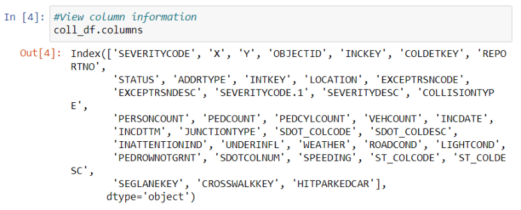
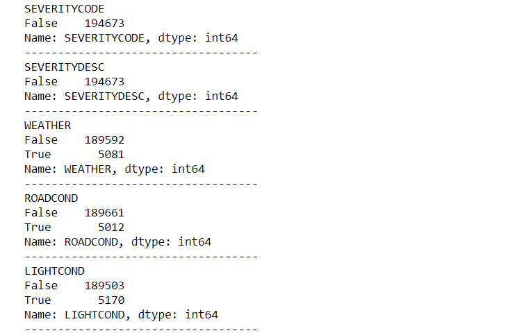
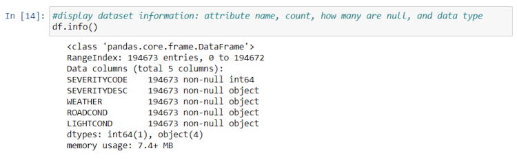
In this project, shared data for Seattle city from Applied Data Science Capstone Project Week1 are used [4]. The dataset consists of 38 columns, 35 columns are the attributes or independent variables. One column* (column A and N) is the dependent or the predicted variable, SEVERITYCODE, and another column (column O) is the description of the code, SEVERITYDESC. The predicted variable has two values: either 1 for property damage only collision or 2 for injury collision. The dataset has more than 194,000 records representing all types of collisions provided by Seattle Police Department and recorded by Traffic record in the timeframe 2004 to 2020. This study aims to predict the impact of environmental conditions of the accidents, namely: WEATHER, ROADCAND, and LIGHTCOND. Brief explanation of each attribute can be found in the file uploaded to Github in the link below.

https://github.com/Yusser89/Coursera_Capstone/blob/master/IBMCapstoneProjectWee1_Part2.pdf

• There is a duplicate, column A and Column N both represent SEVERITYCODE

2.1. Feature Selection

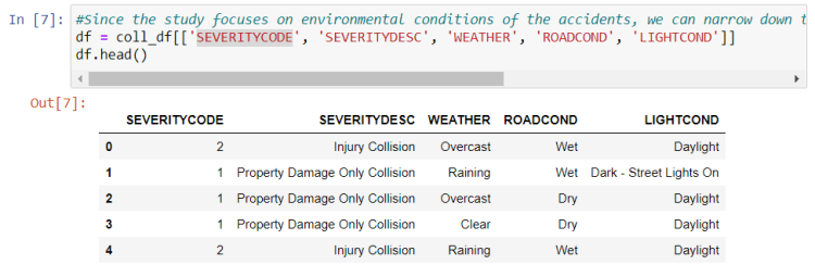
Since the study focuses on environmental conditions of the accidents, we can narrow down the dataset to ‘WEATHER’, ‘ROADCOND’, and ‘LIGHTCOND’.

We begin by importing main libraries followed by loading data file and printing the size of the dataset.

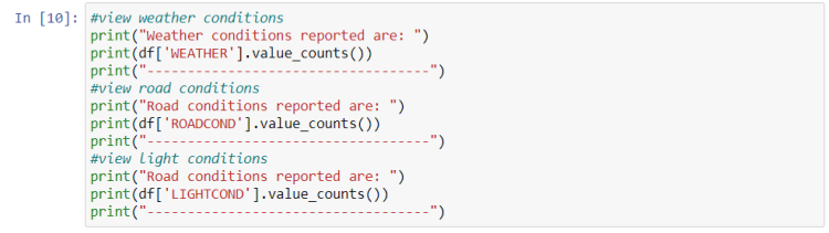
We can view the columns and first five rows of the dataset to get an idea of the data we are dealing with.

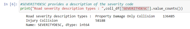
The target variable, ‘SEVERITYCODE’, is described by ‘SEVERITYDESC’. Let’s see how many different codes we have.

So we have two severity codes: 1 for property damage only collision and 2 for injury collision.

We then narrow down our dataset to the features of interest, namely: ‘WEATHER’, ‘ROADCOND’, ‘LIGHTCOND’.

2.2. Handling Missing Data

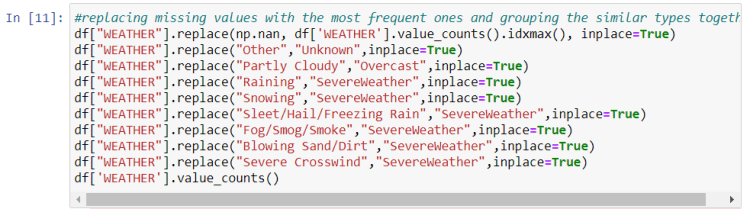
The dataset consists of raw data so there is missing information. First we will search for question marks and replace them with NANs. Then we will replace all NAN values with the most frequent data from each attribute. In addition to that, we are going to group some types of the features together if they are related to each other.

From the results above, it can be seen that we are missing 5081 weather data, 5012 road condition data, and 5170 light condition data. This missing information needs to be addressed.

Trending AI Articles:

1. Fundamentals of AI, ML and Deep Learning for Product Managers

2. The Unfortunate Power of Deep Learning

3. Graph Neural Network for 3D Object Detection in a Point Cloud

4. Know the biggest Notable difference between AI vs. Machine Learning

Let’s also explore the different types of each feature to see if we can group them together

Weather conditions can be grouped as follows:

SevereWeather: Raining, Snowing, Sleet/Hail/Freezing Rain, Fog/Smog/Smoke, Blowing Sand/Dirt, Severe Crosswind
Overcast: PartlyCloudy and Overcast
Unknown: Other

Road conditions can be grouped as follows:

IceOilWaterSnow: Ice, Standing Water, Oil, Snow/Slush, Sand/Mud/Dirt
Unknown: Other

Light conditions can be grouped as follows:

Dark-No-Light: Dark — No Street Lights, Dark — Street Lights Off, Dark — Unknown Lighting
Dark-With-Light: Dark — Street Lights On
DuskDawn: Dusk, Dawn
Unknown: Other

Let’s check if we have any null values

3. Methodology

In this section of the report, exploratory data analysis, inferential statistical testing, and machine learnings used are described.

3.1. Data Visualization

Number of accidents are plotted against each environmental factor (feature) with percentage of each type of each feature to understand the impact of each factor.

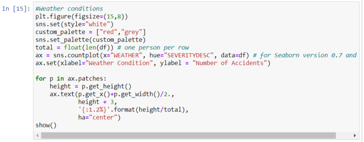
First let’s see the impact of weather conditions.

We can see from the graph above that majority of the accidents happened in clear weather. I was expecting to see more accidents in severe weather.
We need more information on ‘Unknown’ weather conditions as the percentage should not be neglected particularly for accidents that caused property damage only.

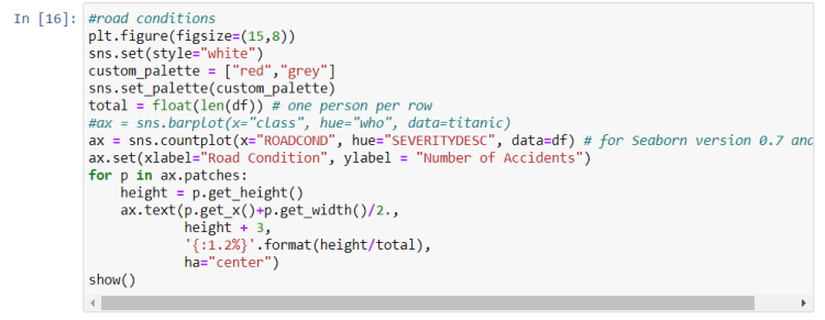
Let’s now see the impact of road conditions.

We can see from the graph above that majority of the accidents happened on dry roads. I was expecting to see more accidents on wet or icy, snowy, oily roads! We also need more information on ‘Unknown’ road conditions as the percentage should not be neglected particularly for accidents that caused property damage only.

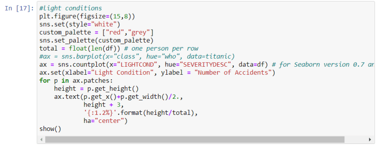
And finally let’s examine the impact of light conditions.

It can be seen from the graph above that majority of accidents happened during the day with daylight. This also was not as I expected! Again, we need more information on ‘Unknown’ light conditions as the percentage should not be neglected particularly for accidents that caused property damage only.

3.2 Machine Learning Model Selection

The preprocessed dataset can be split into training and test sub datasets (70% for training and 30% for testing) using the scikit learn “train_test_split” method. Since the target column (SEVERITYCODE) is categorical, a classification model is used to predict the severity of an accident. Three classification models were trained and evaluated, namely: K-Nearest Neighbor, Decision Tree, and Logistic Regression.

We will start by defining the X (independent variables) and y (dependent variable) as follows.

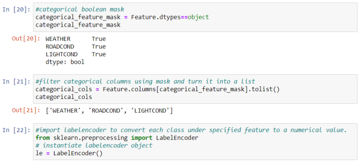
X data needs to be converted to numerical data to be used in the classification models. This can be achieved by using Label Encoding.

It is always better to normalize the features data.

3.2.1. Model

It’s time to build our models by first splitting our data into training and testing sets of 70% and 30% respectively.

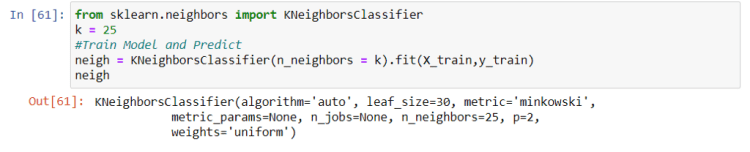
3.2.1.1. K Nearest Neighbor(KNN)

KNN is used to predict the severity of an accident of an unknown dataset based on its proximity in the multi-dimensional hyperspace of the feature set to its “k” nearest neighbors, which have known outcomes. Since finding the best k is memory-consuming and time-consuming, we will use k=25 based on [5].

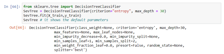
3.2.1.2. Decision Tree

A decision tree model is built from historical data of accident severity in relationship to environmental conditions. Then the trained decision tree can be used to predict the severity of an accident. Since finding the maximum depth is also memory and time consuming, will use max_depth=30 based on [5].

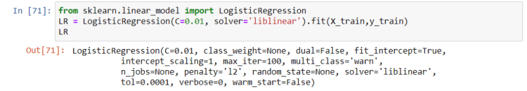
3.2.1.3. Logistic Regression

Logistic Regression is useful when the observed dependent variable, y, is categorical. It produces a formula that predicts the probability of the class label as a function of the independent variables. An inverse-regularisation strength of C=0.01 is used as in [5].

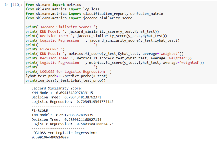
4. Results (Model Evaluation)

Accuracy of the 3 models is calculated using these metrics: Jaccard Similarity Score, F1-SCORE, and LOGLOSS (with Linear Regression).

5. Discussion

First the dataset had categorical data of type ‘object’. Label encoding was used to convert categorical features to numerical values. The imbalanced data issue was ignored because there was a problem installing imbalanced-learn to use imblearn.

Once data was cleaned and analyzed, it was fed into three ML models: K-Nearest Neighbor, Decision Tree, and Logistic Regression. Values of k, max depth and inverse-regularisation strength C were taken from [5]. Evaluation metrics used to test the accuracy of the models were Jaccard Similarity Index, F-1 SCORE and LOGLOSS for Logistic Regression.

It is highly recommended to solve the data imbalance problem for more accurate results.

6. Conclusion

The goal of this project is to analyze historical vehicle crash data to understand the correlation of environmental conditions (weather, road surface, and lighting conditions) with accident severity. Vehicle accident data from the City of Seattle’s’ Police Department for the years 2004 until present were Used. The data was cleaned, and features related to environmental conditions were selected and analyzed. It was found that majority of accidents happened in clear weather, dry roads, and during daytime which wasn’t what I expected. Machine learning models; K-Nearest Neighbor, Decision Tree and Logistic Regression were used to predict the severity of an accident based on certain environmental conditions. The models used were also evaluated using different accuracy metrics.

7. References

1. Road Traffic Injuries and Deaths — A Global Problem. CDC, Center for Disease Control and Prevention, https://www.cdc.gov/injury/features/global-road-safety/index.html#:~:text=Road%20traffic%20crashes%20are%20a,citizens%20residing%20or%20traveling%20abroad.
2. Road Traffic Injuries. WHO, Global Health Observation Data, https://www.who.int/health-topics/road-safety#tab=tab_1
3. Car Accident Statistics in the U.S. Driver Knowledge, https://www.driverknowledge.com/car-accident-statistics/#:~:text=U.S.%20every%20year%20is%206,experience%20permanent%20injuries%20every%20year
4. Shared data for Seattle city from Applied Data Science Capstone Project Week1, https://s3.us.cloud-object-storage.appdomain.cloud/cf-courses-data/CognitiveClass/DP0701EN/version-2/Data-Collisions.csv
5. Seattle Car Accident Severity — IBM Capstone Project by AP Thomson, https://medium.com/@alasdair.p.thomson/seattle-car-accident-severity-ibm-capstone-project-9cef20fc7e6adn

Thank you for reading!

Yusser Al-Qazwini

Don’t forget to give us your ? !

IBM Data Science Capstone: Car Accident Severity Report was originally published in Becoming Human: Artificial Intelligence Magazine on Medium, where people are continuing the conversation by highlighting and responding to this story.

Via https://becominghuman.ai/ibm-data-science-capstone-car-accident-severity-report-a1d2f5070d96?source=rss—-5e5bef33608a—4

I took this problem statement from Kaggle competition. Here we have two datasets.

1. True.csv
2. Fake.csv

So let’s work with these datasets in collab. You can access my repository mentioned bottom of this blog.

Let’s jump directly in coding.

Primary Steps

1. Import all the necessary libraries.

import numpy as np

import pandas as pd

import seaborn as sns

import matplotlib.pyplot as plt

import nltk,re,string,unicodedata

from nltk import pos_tag

from nltk.corpus import wordnet,stopwords

from nltk.stem.porter import PorterStemmer

from wordcloud import WordCloud,STOPWORDS

from nltk.stem import WordNetLemmatizer

from nltk.tokenize import word_tokenize,sent_tokenize

from bs4 import BeautifulSoup

import keras

import tensorflow as tf

from keras.preprocessing import text, sequence

from sklearn.metrics import classification_report,confusion_matrix,accuracy_score

from sklearn.preprocessing import LabelBinarizer

from sklearn.model_selection import train_test_split

from string import punctuation

from keras.models import Sequential

from keras.layers import Dense,Embedding,LSTM,Dropout

from keras.callbacks import ReduceLROnPlateau

2. Load both the datasets.

true_dataset = pd.read_csv(“True.csv”)

false_dataset = pd.read_csv(“Fake.csv”)

3. Check and analyse both the datasets.

4. Creating a new column with name “category”, and assigning “0″ for false news whereas “1” for true news.

true_dataset[‘category’] = 1

false_dataset[‘category’] = 0

5. Now we need to merge both the datasets together.

dataset = pd.concat([true_dataset,false_dataset])

6. Let’s analyse the final dataset.

Data Preprocessing

In the final dataset, we don’t need few columns like “title”, “subject”, “date”. So we are going to remove them.

dataset[‘text’] = dataset[‘text’] + “ “ + dataset[‘title’]

del dataset[‘title’]

del dataset[‘subject’]

del dataset[‘date’]

Now we need to download stopwords from NLTK.

nltk.download(‘stopwords’)

stop = set(stopwords.words(‘english’))

punctuation = list(string.punctuation)

stop.update(punctuation)

Here we are going to create our own functions for doing preprocessing of our data.

def strip_html(text):

soup = BeautifulSoup(text, “html.parser”)

return soup.get_text()

#Removing the square brackets

def remove_between_square_brackets(text):

return re.sub(‘\[[^]]*\]’, ‘’, text)

# Removing URL’s

def remove_between_square_brackets(text):

return re.sub(r’http\S+’, ‘’, text)

#Removing the stopwords from text

def remove_stopwords(text):

final_text = []

for i in text.split():

if i.strip().lower() not in stop:

final_text.append(i.strip())

return “ “.join(final_text)

#Removing the noisy text

def denoise_text(text):

text = strip_html(text)

text = remove_between_square_brackets(text)

text = remove_stopwords(text)

return text

#Apply function on review column

dataset[‘text’]=dataset[‘text’].apply(denoise_text)

Trending AI Articles:

1. Fundamentals of AI, ML and Deep Learning for Product Managers

2. The Unfortunate Power of Deep Learning

3. Graph Neural Network for 3D Object Detection in a Point Cloud

4. Know the biggest Notable difference between AI vs. Machine Learning

Data Visualization

1. Count Plot

sns.set_style(“darkgrid”)

sns.countplot(dataset.category)

2. Sub Plot

fig,(ax1,ax2)=plt.subplots(1,2,figsize=(12,8))

text_len=dataset[dataset[‘category’]==1][‘text’].str.len()

ax1.hist(text_len,color=’red’)

ax1.set_title(‘Original text’)

text_len=dataset[dataset[‘category’]==0][‘text’].str.len()

ax2.hist(text_len,color=’green’)

ax2.set_title(‘Fake text’)

fig.suptitle(‘Characters in texts’)

plt.show()

fig,(ax1,ax2)=plt.subplots(1,2,figsize=(12,8))

text_len=dataset[dataset[‘category’]==1][‘text’].str.split().map(lambda x: len(x))

ax1.hist(text_len,color=’red’)

ax1.set_title(‘Original text’)

text_len=dataset[dataset[‘category’]==0][‘text’].str.split().map(lambda x: len(x))

ax2.hist(text_len,color=’green’)

ax2.set_title(‘Fake text’)

fig.suptitle(‘Words in texts’)

plt.show()

fig,(ax1,ax2)=plt.subplots(1,2,figsize=(20,10))

word=dataset[dataset[‘category’]==1][‘text’].str.split().apply(lambda x : [len(i) for i in x])

sns.distplot(word.map(lambda x: np.mean(x)),ax=ax1,color=’red’)

ax1.set_title(‘Original text’)

word=dataset[dataset[‘category’]==0][‘text’].str.split().apply(lambda x : [len(i) for i in x])

sns.distplot(word.map(lambda x: np.mean(x)),ax=ax2,color=’green’)

ax2.set_title(‘Fake text’)

fig.suptitle(‘Average word length in each text’)

Now we’ll split our dataset into training and testing.

x_train,x_test,y_train,y_test = train_test_split(dataset.text,dataset.category,random_state = 0)

Creating Model

Tokenizing

max_features = 10000

maxlen = 300

tokenizer = text.Tokenizer(num_words=max_features)

tokenizer.fit_on_texts(x_train)

tokenized_train = tokenizer.texts_to_sequences(x_train)

x_train = sequence.pad_sequences(tokenized_train, maxlen=maxlen)

tokenized_test = tokenizer.texts_to_sequences(x_test)

X_test = sequence.pad_sequences(tokenized_test, maxlen=maxlen)

Embedding

EMBEDDING_FILE = ‘glove.twitter.27B.100d.txt’

Model

#LSTM

model = Sequential()

model.add(Embedding(max_features, output_dim=embed_size, weights=[embedding_matrix], input_length=maxlen, trainable=False))

model.add(LSTM(units=128 , return_sequences = True , recurrent_dropout = 0.25 , dropout = 0.25))

model.add(LSTM(units=64 , recurrent_dropout = 0.1 , dropout = 0.1))

model.add(Dense(units = 32 , activation = ‘relu’))

model.add(Dense(1, activation=’sigmoid’))

model.compile(optimizer=keras.optimizers.Adam(lr = 0.01), loss=’binary_crossentropy’, metrics=[‘accuracy’])

Summary of our model

model.summary()

Fitting the model

history = model.fit(x_train, y_train, batch_size = batch_size , validation_data = (X_test,y_test) , epochs = epochs , callbacks = [learning_rate_reduction])

Accuracy of the model

You can clone my repository from here. And can also work with this dataset and can come with another approach.

Don’t forget to give us your ? !

Machine Learning Model for Detecting Fake News. was originally published in Becoming Human: Artificial Intelligence Magazine on Medium, where people are continuing the conversation by highlighting and responding to this story.

Via https://becominghuman.ai/machine-learning-model-for-detecting-fake-news-cae28a8574ef?source=rss—-5e5bef33608a—4