365 Data Science

The curious mind wanders

In my life, I’m very creative, but the cost of creativity, for me, has been focus. I’m curious to a fault, and while that has been the drive behind taking too many classes in school, it has also hindered my ability to be productive. That’s not to say I haven’t had major finds as a results; I have. I don’t think creativity and focus have to be all or nothing. I’ve been working on maintaining a balance to not only maintain a job but also to find the best, most impacting ideas.

In high school, I definitely had this problem in class. The material was always interesting to me, but my ability to remain focused got in the way of some good essay writing. This was especially true in my history class where we would have to write one essay a week, and while I loved the material, I was scatter brained when pen went to paper. Strange to think that now I read a few history books a year.

In college, it turns out I’m very capable at math which means I didn’t need to study so much. However, the downside is that I didn’t go into as much depth on some materials as I would have liked. For my senior design project, I really let loose in designing the computer vision system for our autonomous vehicle. I mostly wrote the code on my own, and I got very creativity in using uint16 instead of float to shave off some valuable seconds of the processing time. However, I didn’t quite have the focus to comment my code appropriately, even though it was highly efficient code. The end result is that my code was not used by anyone else, which I regret.

At Notre Dame, I quickly learned my motivation was to graduate on time. This meant I had to focus. I determined when I wanted to finish, and I back tracked all the time requirements of each module of my work. The result was that I had a rough idea of when things had to get done, and this allowed me to stay more or less on track.

At DSC, I had a mixed bag. When I started, we were only using the entire face (as opposed to regions) for face recognition when the literature at the time suggested any method would be improved by multiple regions fused together. My manager had other things for me to work on, but I kept getting drawn to this low hanging fruit. To even do the testing, I revamped the code and sped it up by a factor of 10. I was using the oldest computer at the company, so my code needed to run just a bit faster if I wanted to do the experiments properly. I threw together a few rough regions, and I was able to quickly show how much more improvement one got form multiple face regions. After that, my previous tasks went out the window, and while I was happy, I’m sure it was frustrating to my manager.

Trending AI Articles:

1. Fundamentals of AI, ML and Deep Learning for Product Managers

2. The Unfortunate Power of Deep Learning

3. Graph Neural Network for 3D Object Detection in a Point Cloud

4. Know the biggest Notable difference between AI vs. Machine Learning

On the other hand, when I came up with a method for improve the 3D depth quality by upsampling, I spent two months of my time implementing the method in C++ that was unnecessary. I had been trying to implement the more complex methods of upsampling (based on the griddata function in Matlab) when in fact, I had found major gains using the least complex. I was stubborn in part because of my curiosity on how to efficiently implement these higher order methods. Finally, I turned my work full force on getting the basic method implemented, and I was able to achieve a certain level of focus.

At Apple, on the Watch, my creativity lead to a breakthrough in background heart rate. Two months later, I received feedback about the previous year (before this breakthrough) that I was not focused enough. I couldn’t deny the claim. I had been working on Wrist Detection, and certainly I had times where I went off on a tangent. However, my argument had been the saving grace of my creativity. I would still argue that my creativity was worth a lack of focus, and I would go so far as to say I could not do both.

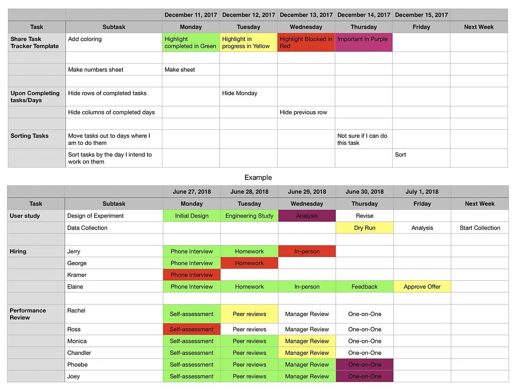
On Face ID, that changed in part because of the volume of tasks and task switching. I was compelled to find a better way to track progress on different tasks and also not drop any of them. This started with a Notepad document that turned into a Word document, and that morphed into a Numbers sheet. I was able to add in my ideas of curiosity into my sheet so I would not forget them, but I could also see the other work I had to do and prioritize accordingly. Suddenly, I was able to stay focused and switch focuses quicker just by knowing where I was on a project. This didn’t seem to dampen my ability to be highly creative in trying to solve problems either.

I’m still working on the balance, and I believe this is key to hitting a maximum potential. I have ideas all the time, but that doesn’t mean they are all good. It just means I have so much to throw against the wall, one of them is bound to stick.

If you like, follow me on Twitter and YouTube where I post videos espresso shots on different machines and espresso related stuff. You can also find me on LinkedIn.

Further readings of mine:

Data Science: Essentials

Abandon Ship: How a startup went under

Dissertation Regret

Part of the Team

How to Interview a Company

Thoughts on Leaving

A Day in the Life of a Data Scientist

Design of Experiment: Data Collection

Don’t forget to give us your ? !

Balancing Creativity and Focus was originally published in Becoming Human: Artificial Intelligence Magazine on Medium, where people are continuing the conversation by highlighting and responding to this story.

Via https://becominghuman.ai/balancing-creativity-and-focus-578db1332dfb?source=rss—-5e5bef33608a—4

DengAI: Predicting Disease Spread — Imputation and Stationary Problems

Github Repository

One of the biggest data challenge on DrivenData, with more than 9000 participants is the DengAI challenge. The objective of this challenge is predict the number of dengue fever cases in two different cities.

This blogpost series covers our journey of tackling this problem, starting from initial data analysis, imputation and stationarity problems up un to the different forecasting attempts. This first post covers the imputation and stationarity checks for both cities in the challenge, before moving on to trying different forecasting methdologies.

Throughout this post, code-snippets are shown in order to give an understanding of how the concepts discussed are implemented into code. The entire Github repository for the imputation and stationary adjustment can be found here.

Furthermore, in order to ensure readability we decided to show graphs only for the city San Jose instead showing it for both cities.

Imputation

Imputation describes the process of filling missing values within a dataset. Given the wide range of possibilities for imputation and the severe amount of missing data within this project, it is worthwhile to go over some of the methods and empirically check which one to use.

Overall, we divide all imputation methods into the two categories: basic and advanced. With basic methods we mean off the shelf, quick imputation methods, which are oftentimes already build into Pandas. Advanced imputation methods deal with model-based approaches where the missing values are attempted to be predicted, using the remaining columns.

Given that the model-based imputation methods normally result in superior performance, the question might arise why we do not simply use the advanced method for all columns. The reason for that is that our dataset has several observations where all features are missing. The presence of these observations make multivariate imputation methods impossible.

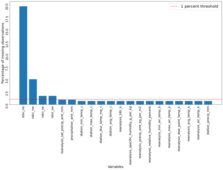
We therefore divide the features into two categories. All features, or columns, which have fewer than 1 percent missing observations are imputed using more basic methods, whereas model-based approaches are used for features which exhibit more missing observations than this threshold.

The code snippet below counts the percentage of missing observations, divides all features into one of two aforementioned categories and creates a graph to visualize the results.

The resulting graph below shows four features which have more than 1 percent of observations missing. Especially the feature ndvi_ne, which describes satellite vegetation in the north-west of the city has a severe amount of missing data, with more around 20% of all observation missing.

Trending AI Articles:

1. Fundamentals of AI, ML and Deep Learning for Product Managers

2. The Unfortunate Power of Deep Learning

3. Graph Neural Network for 3D Object Detection in a Point Cloud

4. Know the biggest Notable difference between AI vs. Machine Learning

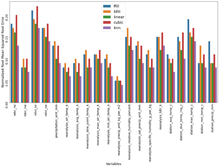
All imputation methods applied are compared using the normalized root mean squared error (NRMSE). We use this quality estimation method because of its capability for making variables with different scales comparable. Given that the NRMSE is not directly implemented in Python, we use the following snippet to implement it.

Basic imputation methods

Python, and in particular the library Pandas, has multiple off-the-shelf imputation methods available. Arguably the most basic ones are forward fill (ffill) and backward fill (bfill), where we simply set the missing valueequal to the prior value (ffill) or to the proceeding value (bfill).

Other methods include the linear or cubic (the Scipy package also includes higher power if wanted) interpolation around a missing observation.

Lastly, we can use the average of the k nearest neighbours of a missing observations. For this problem we took the preceding and proceeding four observations of a missing observation and imputed it with the average of these eight values. This is not a build in method and therefore defined by us in the following way:

Now it is time to apply and compare of these methods. We do that by randomly dropping 50 observations of all columns, which are afterwards imputed by all before mentioned methods. Afterwards we assess each method’s performance through their NRMSE score. All of that, and the graphing of the results is done through the following code snippet.

The resulting graph below clearly shows which method is to be favored, namely the k nearest neighbours approach. The linear method also performs well, even though not as well as the knn method. The more naive methods like ffill and bfill do not perform as strongly.

Afterwards, we impute all features which had fewer observations missing than our threshold of one percent. That means all features except the first four. The code below selects the best method for each column and afterwards imputes all actual missing values.

The potential flaws of the knn approach

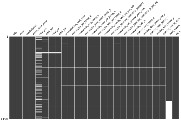
Unfortunately, the superior performance of the knn model comes with a price. For some features, we do not have a only one observation missing at a time, but multiple consecutively missing observations.

If for example we have 12 consecutive missing observations, the knn method cannot calculate any average out of the preceding and proceeding four observations, given that they are missing as well.

The image below, which was created with the beatiful missingno package, shows us that all four columns which were classified as being above our one percent threshold have at one point 15 consecutive missing observations. This makes it impossible to use the knn method for these columns and is the reason why we cannot use this imputation method for the heavily sparse columns.

Model-based imputation methods

The model-based imputation methods use, as already described earlier, the column with the missing observations as the target and uses all other possible columns as the features. After imputing all columns with fewer than one percent missing observations, we can now use all of them as features.

The model we are using is a RandomForestRegressor because of its good handling of noisy data. The code snippet below which hyperparameters were gridsearched.

imputation_model = {
        "model": RandomForestRegressor(random_state=28),
        "param": {
            "n_estimators": [100],
            "max_depth": [int(x) for x in
                          np.linspace(10, 110, num=10)],
            "min_samples_split": [2, 5, 10, 15, 100],
            "min_samples_leaf": [1, 2, 5, 10]
            }
        }

We now run all four columns through the model-based approach and compare their performance to all aforementioned basic imputation methods. The following code snippet takes care of exactly that.

Below we can see that our work was worthwhile. For three out of four columns we find a superior performance of the model-based approach compared to the basic imputation methods. We are now left with a fully imputed dataset with which we can proceed.

Stationarity Problems — Seasonality and Trend

In contrast to cross-sectional data, time series data comes with a whole bunch of different problems. Undoubtedly one of the biggest issues is the problem of stationarity. Stationarity describes a measure of regularity. It is this regularity which we depend on to exploit when building meaningful and powerful forecasting models. The absence of regularity makes it difficult at best to construct a model.

There are two types of stationarity, namely strict and covariance stationarity. In order for a time series to be fulfil strict stationarity, the series needs to be time independent. That would imply that the relationship between two observations of a series is only driven by the timely gap between them, but not on the time itself. This assumption is difficult, if not impossible for most time series to meet and therefore more focus is drawn on covariance stationarity.

For a time series to be covariance stationary, it is required that the unconditional first two moments, so the mean and variance, are finite and do not change with time. It is important to note that the time series is very much allowed to have a varying conditional mean. Additionally, it is required that the auto-covariance of a time series is only depending on the lag number, but not on the time itself. All these requirements are also stated below.

There are many potential reasons for a time series to be non-stationary, including seasonalities, unit roots, deterministic trends and structural breaks. In the following section we will check and adjust our exogenous variable for each of these criteria to ensure stationarity and superior forecasting behavior.

Seasonality

Seasonality is technically a form of non-stationarity because the mean of the time series is dependent on time factor. An example would be the spiking sales of a gift-shop around Christmas. Here the mean of the time series is explicitly dependent on time.

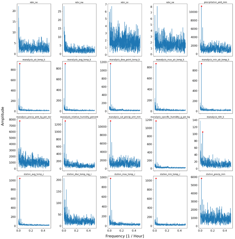
In order to adjust for seasonality within our exogenous variables, we first have to find out which variables actually exhibits that kind of behavior. This is done by applying a Fourier Transform. A Fourier transform disentangles a signal into its different frequencies and assesses the power of each individual frequency. The resulting plot, which shows power as a function of frequency is called a power spectrum. The frequency with the strongest power could then be potentially the driving seasonality in our time series. More information about Fourier transform and signal processing in general can be read up on an earlier blogpost of ours here.

The following code allows us to take a look into the power-plots of our 20 exogenous variable.

The plot below shows the resulting 20 exogenous variables. Whether or not a predominant and significant threshold is met for a variable is indicated by a red dot on top of a spike. If a red dot is visible, that means that the time series has a significantly driving frequency and therefore a strong seasonality component.

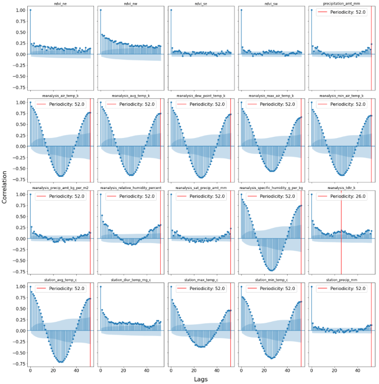
One possibility to cross-check the results of the Fourier Transforms is to plot the Autocorrelation function. If we would try have a seasonality of order X, we would expect a significant correlation with lag X. The following snippet of code plots the autocorrelation function for all features and highlights those features which are found to have a seasonal affect according to the Fourier Transform.

From the ACF plots below, we can extract a lot of useful information. First of all, we can clearly see that for all columns where the Fourier transforms find a significant seasonality, we also find confirming picture. This is because we see a peaking and significant autocorrelation at the lag which was found by the power-plot.

Additionally, we find some variables (e.g. ndvi_nw) which exhibit a constant significant positive autocorrelation. This is a sign of non-stationarity, which will be addressed in the next section which will be dealing of stochastic and deterministic trends.

In order to get rid of the seasonal component, we decompose each seasonality-affected feature into its unaffected version its seasonality component and trend component. This is done by the STL decomposition which was developed by Cleveland, McRae & Terpenning (1990). STL is an acronym for “Seasonal and Trend decomposition using Loess”, while Loess is a method for estimating non-linear relationships.

The following code snippet decomposes the relevant time series, and subtracts (given that we face additive seasonalities) the seasonality and the trend from the time series.

Deterministic Trends

One more obvious way to breach the assumptions of covariance stationarity is if the series has a deterministic trend. It is important to stress the difference between a deterministic and not a stochastic trend (unit root). Whereas it is possible to model and remove a deterministic trend, this is not possible with a stochastic trend, given its unpredictable and random behavior.

A deterministic trend is the simplest form of a non-stationary process and time series which exhibit such a trend can be decomposed into three components:

The most common type of trend is a linear trend. It is relatively straight forward to test for such a trend and remove it, if one is found. We apply the original Mann-Kendall test, which does not consider seasonal effects, which we already omitted in the part above. If a trend is found, it is simply subtracted from the time series. These steps are completed in the method shown below.

The result can be viewed here. As we can see, most time series exhibited a linear trend, which was then removed.

Even though we removed a deterministic trend, this did not ensure that our time series are actually stationary now. That is because what works for a deterministic trend does not work for a stochastic trend, meaning that the trend-removing we just did does not ensure stationary of unit-roots.

We therefore have to explicitly test for a unit-root in every time series.

Stochastic Trends — Unit roots

A unit root process is the generalization of the classic random walk, which is defined as the succession of random steps. Given this definition, the problem of estimating such a time series are obvious. Furthermore, a unit root process violates the covariance stationarity assumptions of not being dependent on time.

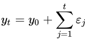
To see why that is the case, we assume an autoregressive model where today’s value only depends on yesterday’s value and an error term.

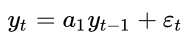
If we parameter a_1 would now be equal to one, the process would simplify to

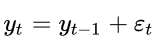
By repeated substitution we could also write this expression as:

When now calculating the variance of y_t, we face a variance which is positively and linearly dependent on time, which violates the second covariance stationarity rule.

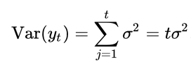
This would have not been the case if a_1 would be smaller than one. That is also basically what is tested in an unit-root test. Arguably the most well-known test for an unit root is the Augmented Dickey Fuller (ADF) test. This test has the null hypothesis of having a unit root present in an autoregressive model. The alternative is normally that the series is stationary or trend-stationary. Given that we already removed a (linear) trend, we assume that the alternative is a stationary series.

In order to be technically correct, it is to be said that the ADF test is not directly testing that a_1 is equal to zero, but rather looks at the characteristic equation. The equation below illustrates what is meant by that:

We can see that the difference to the equation before is that we do not look at the level of y_t, but rather at the difference of y_t. Capital Delta represent here the difference operator. The ADF is now testing whether the small delta operator is equal to zero. If that would not be the case, then the difference between yesterday’s and tomorrow’s value would depend on yesterday’s value. That would mean if the today’s value is high, the difference between today’s and tomorrow’s value will also be large which is a self-enforcing and explosive process which clearly depends on time and therefore breaks the assumptions of covariance stationarity.

In case of a significant unit-root (meaning a pvalue above 5%), we difference the time series as often as necessary until we find a stationary series. All of that is done through the following two methods.

The following table shows that we do not find any significant ADF test, meaning that no differencing was needed and that no series exhibited a significant unit root.

Finishing up

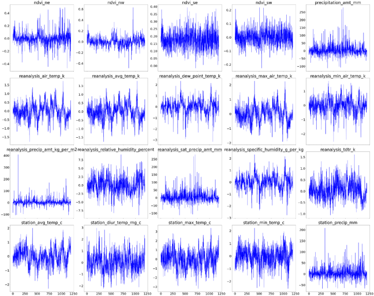
Last but not least we take a look at our processed time series. It is nicely visible that none of the time series are trending anymore and they do not exhibit significant seasonality anymore.

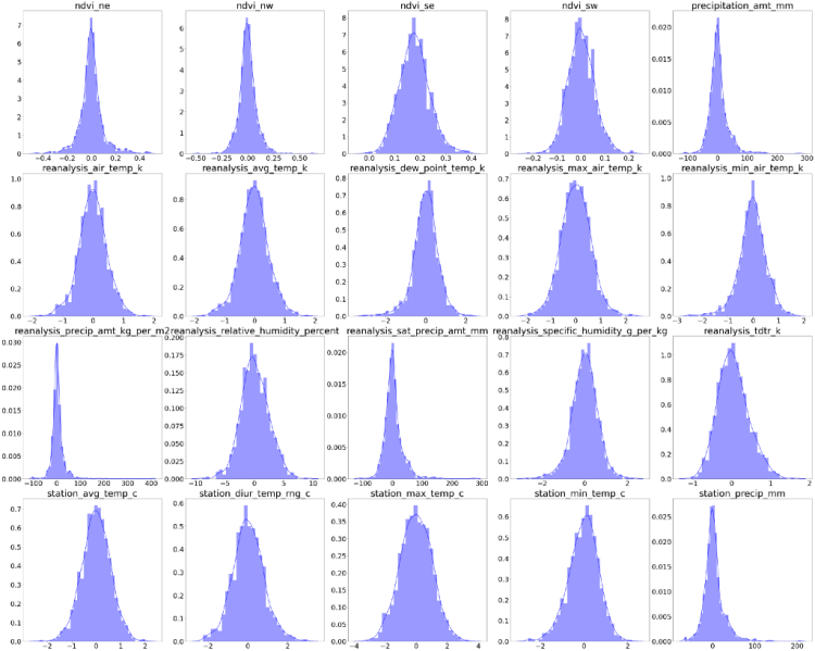
Additionally we take a look at how the distributions of all of the series look. It is important to note that there are no distributional assumptions of the feature variables when it comes to forecasting. That means that even if we find highly skewed variables, it is not necessary to apply any transformation.

After sufficiently transforming all exogenous variables, it is now time to shift our attention on the forecasting procedure of both cities.

Don’t forget to give us your ? !

DengAI: Predicting Disease Spread — Imputation and Stationary Problems was originally published in Becoming Human: Artificial Intelligence Magazine on Medium, where people are continuing the conversation by highlighting and responding to this story.

Via https://becominghuman.ai/dengai-predicting-disease-spread-imputation-and-stationary-problems-f08c7bac06f1?source=rss—-5e5bef33608a—4