365 Data Science

Via https://becominghuman.ai/google-analysis-of-online-dataset-4f25db2951ef?source=rss—-5e5bef33608a—4

Via https://becominghuman.ai/why-do-people-use-python-a4e0fcd2575d?source=rss—-5e5bef33608a—4

We are going to show how we can estimate card probabilities by applying Monte Carlo Simulation and how we can solve them numerically in Python. The first thing that we need to do is to create a deck of 52 cards.

How to Generate a Deck of Cards

import itertools, random

# make a deck of cards
deck = list(itertools.product(['A', '2', '3', '4', '5', '6', '7', '8', '9', '10', 'J', 'Q', 'K'],['Spade','Heart','Diamond','Club']))

deck

And we get:

[('A', 'Spade'),
 ('A', 'Heart'),
 ('A', 'Diamond'),
 ('A', 'Club'),
 ('2', 'Spade'),
 ('2', 'Heart'),
 ('2', 'Diamond'),
 ('2', 'Club'),
 ('3', 'Spade'),
 ('3', 'Heart'),
 ('3', 'Diamond'),
 ('3', 'Club'),
 ('4', 'Spade'),
 ('4', 'Heart'),
 ('4', 'Diamond'),
 ('4', 'Club'),
 ('5', 'Spade'),
 ('5', 'Heart'),
...

]

How to Shuffle the Deck

# shuffle the cards
random.shuffle(deck)
deck[0:10]

And we get:

[('6', 'Club'),
 ('8', 'Spade'),
 ('J', 'Heart'),
 ('10', 'Heart'),
 ('Q', 'Spade'),
 ('7', 'Diamond'),
 ('K', 'Diamond'),
 ('J', 'Club'),
 ('J', 'Diamond'),
 ('A', 'Club')]

How to Sort the Deck

For some probabilities where the order does not matter, a good trick is to sort the cards. The following commands can be helpful.

# sort the deck
sorted(deck)

# sort by face
sorted(deck, key = lambda x: x[0])

# sort by suit
sorted(deck, key = lambda x: x[1])

How to Remove Cards from the Deck

Depending on the Games and the problem that we need to solve, sometimes there is a need to remove from the Deck the cards which have already been served. The commands that we can use are the following:

# assume that card is a tuple like ('J', 'Diamond')
deck.remove(card)

# or we can use the pop command where we remove by the index
deck.pop(0)

# or for the last card
deck.pop()

Trending AI Articles:

1. Microsoft Azure Machine Learning x Udacity — Lesson 4 Notes

2. Fundamentals of AI, ML and Deep Learning for Product Managers

3. Roadmap to Data Science

4. Work on Artificial Intelligence Projects

Part 1: Estimate Card Probabilities with Monte Carlo Simulation

Question 1: What is the probability that when two cards are drawn from a deck of cards without a replacement that both of them will be Ace?

Let’s say that we were not familiar with formulas or that the problem was more complicated. We could find an approximate probability with a Monte Carlo Simulation (10M Simulations)

N = 10000000
double_aces = 0

for hands in range(N):
    # shuffle the cards
    random.shuffle(deck)
    aces = [d[0] for d in deck[0:2]].count('A')
    if aces == 2:
        double_aces+=1

prob = double_aces/N
prob

And we get 0.0045214 where the actual probability is 0.0045

Question 2: What is the probability of two Aces in 5 card hand without replacement.

FYI: In case you want to solve it explicitly by applying mathematical formulas:

from scipy.stats import hypergeom

# k is the number of required aces
# M is the total number of the cards in a deck
# n how many aces are in the deck
# N how many aces cards we will get

hypergeom.pmf(k=2,M=52, n=4, N=5)

And we get 0.03992981808107859. Let’s try to solve it by applying simulation:

N = 10000000
double_aces = 0

for hands in range(N):
    # shuffle the cards
    random.shuffle(deck)
    aces = [d[0] for d in deck[0:5]].count('A')
    if aces == 2:
        # print(deck[0:2])
        double_aces+=1

prob = double_aces/N
prob

And we get 0.0398805. Again, quite close to the actual probability

Question 3: What is the probability of being dealt a flush (5 cards of all the same suit) from the first 5 cards in a deck?

If you would like to see the mathematical solution of this question you can visit PredictiveHacks. Let’s solve it again by applying a Monte Carlo Simulation.

N = 10000000

flushes = 0

for hands in range(N):
    # shuffle the cards
    random.shuffle(deck)
    flush = [d[1] for d in deck[0:5]]
    if len(set(flush))== 1:
        flushes+=1
prob = flushes/N
prob

And we get 0.0019823 which is quite close to the actual probability which is 0.00198.

Question 4: What is the probability of being dealt a royal flush from the first 5 cards in a deck?

The actual probability of this case is around 0.00000154. Let’s see if the Monte Carlo works with such small numbers.

# royal flush

N = 10000000
royal_flushes = 0
for hands in range(N):
    # shuffle the cards
    random.shuffle(deck)
    flush = [d[1] for d in deck[0:5]]
    face = [d[0] for d in deck[0:5]]
    if len(set(flush))== 1 and sorted(['A','J', 'Q', 'K', '10'])==sorted(face):
    royal_flushes+=1

prob = royal_flushes/N
prob

And we get 1.5e-06 which is a very good estimation.

Part 2: Calculate Exact Card Probabilities Numerically

Above, we showed how we can calculate the Card Probabilities explicitly by applying mathematical formulas and how we can estimate them by applying Monte Carlo Simulation. Now, we will show how we can get the exact probability using Python. This is not always applicable but let’s try to solve the questions of Part 1.

The logic here is to generate all the possible combinations and then to calculate the ratio. Let’s see how we can get all the possible 5-hand cards of a 52-card deck.

# importing modules

import itertools
from itertools import combinations

# make a deck of cards
deck = list(itertools.product(['A', '2', '3', '4', '5', '6', '7', '8', '9', '10', 'J', 'Q', 'K'], ['Spade','Heart','Diamond','Club']))

# get the (52 5) combinations
all_possible_by_5_combinations = list(combinations(deck,5))

len(all_possible_by_5_combinations)

And we get 2598960 as expected.

Question 1: What is the probability that when two cards are drawn from a deck of cards without a replacement that both of them will be Ace?

# importing modules

import itertools
from itertools import combinations
# make a deck of cards

deck = list(itertools.product(['A', '2', '3', '4', '5', '6', '7', '8', '9', '10', 'J', 'Q', 'K'], ['Spade','Heart','Diamond','Club']))

# get the (52 2) combinations

all_possible_by_2_combinations = list(combinations(deck,2))

Aces = 0

for card in all_possible_by_2_combinations:
    if [d[0] for d in card].count('A') == 2:
        Aces+=1

prob = Aces / len(all_possible_by_2_combinations)
prob

And we get 0.004524886877828055.

Question 2: What is the probability of two Aces in 5 card hand without replacement.

# get the (52 5) combinations

all_possible_by_5_combinations = list(combinations(deck,5))

Aces = 0

for card in all_possible_by_5_combinations:
    if [d[0] for d in card].count('A') == 2:
        Aces+=1

prob = Aces / len(all_possible_by_5_combinations)
prob

And we get 0.03992981808107859

Question 3: What is the probability of being dealt a flush (5 cards of all the same suit) from the first 5 cards in a deck?

# get the (52 5) combinations
all_possible_by_5_combinations = list(combinations(deck,5))

flushes  = 0
for card in all_possible_by_5_combinations:
    flush = [d[1] for d in card]
    if len(set(flush))== 1:
        flushes+=1

prob = flushes / len(all_possible_by_5_combinations)
prob

And we get 0.0019807923169267707

Question 4: What is the probability of being dealt a royal flush from the first 5 cards in a deck?

# get the (52 5) combinations

all_possible_by_5_combinations = list(combinations(deck,5))

royal_flushes   = 0

for card in all_possible_by_5_combinations:
    flush = [d[1] for d in card]
    face = [d[0] for d in card]
    if len(set(flush))== 1 and sorted(['A','J', 'Q', 'K', '10'])==sorted(face):
        royal_flushes +=1

prob = royal_flushes  / len(all_possible_by_5_combinations)
prob

And we get 1.5390771693292702e-06

Discussion

Computing Power enables us to estimate and even calculate complicated probabilities without being necessary to be experts in Statistics and Probabilities. In this post, we provided some relatively simple examples. The same logic can be extended to more advanced and complicated problems in many fields, like simulating card games, lotteries, gambling games etc.

---

Estimate Probabilities Of Card Games was originally published in Becoming Human: Artificial Intelligence Magazine on Medium, where people are continuing the conversation by highlighting and responding to this story.

Via https://becominghuman.ai/estimate-probabilities-of-card-games-3ae50adb75c7?source=rss—-5e5bef33608a—4

You can train your supervised machine learning models all day long, but unless you evaluate its performance, you can never know if your model is useful. This detailed discussion reviews the various performance metrics you must consider, and offers intuitive explanations for what they mean and how they work.

Originally from KDnuggets https://ift.tt/31TVbPP

Check out these 10 things you didn’t know about Scikit-Learn… until now.

Originally from KDnuggets https://ift.tt/3hVpprf

Also: Full Stack #DeepLearning course; Guide to Intelligent #DataScience book – updated/expanded content throughout, now an even better basis for the “educational” part of “becoming a successful data scientist”; Completely Free #MachineLearning Reading List by @vickdata; A Complete #DataScience Portfolio Project

Originally from KDnuggets https://ift.tt/31Q0rE8

Learn what is data enrichment, what are the different types, benefits and use cases for data enrichment, and how SmartProxy helps you do it.

Originally from KDnuggets https://ift.tt/3gU53O3

This is an overview of a great computer vision resource from Microsoft, which demonstrates best practices and implementation guidelines for a variety of tasks and scenarios.

Originally from KDnuggets https://ift.tt/2GqOw7P

b News Topic Classification using LSTM

How LSTM (Long Short-Term Memory) cells learn to categorize texts.

Hi everyone, Ardi here. Welcome back to my page! In my last post I was explaining about a simple Exploratory Data Analysis (EDA) and survival prediction on Titanic dataset. Check it out now if you haven’t already!

• Titanic Survival Dataset Part 1/2: Exploratory Data Analysis
• Titanic Survival Dataset Part 2/2: Logistic Regression

Instead of working with a structured dataset again, here I decided to deal with the unstructured one: NLP (Natural Language Processing). To be more precise, in this project I wanna create a neural network architecture which is expected to be able to classify news topics based on its content. The main idea here is to employ LSTM cell thanks to its ability to recognize pattern on sequential data (e.g. signals, texts, etc.)

The dataset that I use for this project is taken from here. If you open the webpage, there will be several download links, and I decided to take the one highlighted in yellow.

It should not take long to download the file since the size of that dataset is only around 14 MB. Now after extracting the compressed file, we should get the following folders:

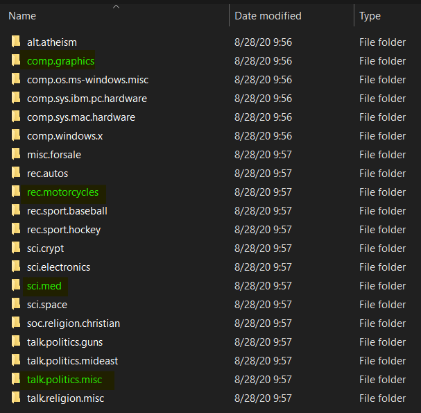
We can see here that there are 20 different classes available in the dataset. However though, in this project I only wanna use 4 of those for the sake of simplicity (the folders that I highlighted in green.)

In total, there are 3732 files in those 4 classes that we use, where each of the first 3 (computer graphics, motorcycles and medical science) consists of approximately 970 samples while the last one (politics) contains around 700 texts.

I do share the final code of this project in the end of this article in Python format (.py). I do recommend you to run it using Jupyter Notebook so that you know exactly what’s actually done at each line. Also, before we go any further, it’s important to ensure that your Python environment is already installed with the following modules:

import os
import re
import numpy as np
import matplotlib.pyplot as plt
import seaborn as sns; sns.set()
from nltk.tokenize import word_tokenize
from nltk.corpus import stopwords
from sklearn.preprocessing import OneHotEncoder
from sklearn.model_selection import train_test_split
from sklearn.metrics import confusion_matrix
from keras.preprocessing import sequence
from keras.preprocessing.text import Tokenizer
from keras.models import Sequential
from keras.layers import Dense, LSTM
from keras.layers.embeddings import Embedding

If there’s no error appears after running those imports above, we should ready to go!

By the way, I divided this article to several chapters:

1. Text preprocessing
2. Label preprocessing
3. Model training
4. Model evaluation

Text preprocessing

The next thing to do after importing all modules is to load the dataset. I am going to create a function called read_file() to make things tidier. This function is pretty simple though. The input is just a path to the text files, while the output is a list in which each of the index holds the content of each file.

# Don't forget to include slash at the end of the path

def read_files(path):
    file_contents = list()
    filenames = os.listdir(path)
    
    for i in range(len(filenames)):
        with open(path+filenames[i]) as f:
            file_contents.append(f.read())
    
    return file_contents

Now we will directly use the function above to read all texts in our dataset like this:

class_0 = read_files('20news-18828/comp.graphics/')
class_1 = read_files('20news-18828/rec.motorcycles/')
class_2 = read_files('20news-18828/sci.med/')
class_3 = read_files('20news-18828/talk.politics.misc/')

Keep in mind that the variables of class_0, class_1, class_2 and class_3 represent computer graphics, motorcycles, medical science and politics labels repsectively. I will also create a labels list which stores each of those class names.

labels = ['comp.graphics', 'rec.motorcycles', 'sci.med', 'talk.politics.misc']

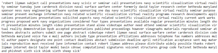
If you wanna check whether our dataset has been loaded successfully, we can print them out. Here I want to print the first article in class_0 by running print(class_0[0]). The output is going to look something like this:

Since all texts are still stored in different array (class_0, class_1, class_2, class_3), we are going to put them all into a single array to simplify our next processes. Here I use np.append() function several times to store everything in all_texts array.

all_texts = np.append(class_0, class_1)
all_texts = np.append(all_texts, class_2)
all_texts = np.append(all_texts, class_3)

Now if we run len(all_texts), then the output will be 3732, in which this value is the total number of files that we are going to work with in this project. However though, it’s important to keep in mind that all these 3732 files are still messy. Thus we need to clean those up using clean() function that I define manually. I also create a stop_words set which contains all stop words in English which I will use them to eliminate all stop words in our dataset.

stop_words = set(stopwords.words('english'))

def clean(text):
    # Lowering letters
    text = text.lower()
    # Removing html tags
    text = re.sub('<[^>]*>', '', text)
    # Removing emails
    text = re.sub('\S*@\S*\s?', '', text)
    # Removing urls
    text = re.sub('https?://[A-Za-z0-9]','',text)
    # Removing numbers
    text = re.sub('[^a-zA-Z]',' ',text)

    word_tokens = word_tokenize(text)    
    filtered_sentence = []
    for word_token in word_tokens:
        if word_token not in stop_words:
            filtered_sentence.append(word_token)
    
    # Joining words
    text = (' '.join(filtered_sentence))
    return text

There are several steps done in the code above. First, the function accepts a raw text as its input. Next, all characters in this raw text is going to be converted into lowercase. This step is very necessary since the exact same words will be interpreted as different words just because one is using lowercase while the other one uses uppercase. HTML tags, email addresses, URLs and numbers are also removed because I think those words are just not quite informative. By the way I use re (Regular Expression) module to get rid of that.

Trending AI Articles:

1. Microsoft Azure Machine Learning x Udacity — Lesson 4 Notes

2. Fundamentals of AI, ML and Deep Learning for Product Managers

3. Roadmap to Data Science

4. Work on Artificial Intelligence Projects

Afterwards, this text is then tokenized using word_tokenize() function taken from NLTK module. What’s essentially done at this tokenization process is that each of the words in the text is going to be put in an array while at the same time all spaces and escape characters (i.e. \t, \n, etc.) are just dropped before eventually the cleaned text is returned.

Now as the clean() function has been created, we are gonna clean all texts and store the result directly to all_cleaned_texts array.

all_cleaned_texts = np.array([clean(text) for text in all_texts])

You may try to run print(all_cleaned_texts[0]) if you wanna see how the cleaned version of our data looks like.

That’s not all of the text preprocessing though! Still we need to encode all those cleaned texts into numbers because we know that all machine learning/deep learning algorithms can only work with numerical data. In order to do that, we are going to employ Tokenizer() object taken from Keras module and use it to create a word-to-number mapping.

tokenizer = Tokenizer()
tokenizer.fit_on_texts(all_cleaned_texts)

We can check how the mapping looks like by taking the word_index attribute of tokenizer object like this:

tokenizer.word_index

It essentially tells us that the word subject is going to be encoded to 1, writes will be 2, and so on. Also, if we try to print out the length of this word_index, then the result will be 35362, where this value represents the number of unique words in our dataset. In this stage, we haven’t actually convert those texts into sequence of numbers. To do that, we still need to run the code below. By the way, I will directly convert that into Numpy array to make future computation easier.

all_encoded_texts = tokenizer.texts_to_sequences(all_cleaned_texts)
all_encoded_texts = np.array(all_encoded_texts)

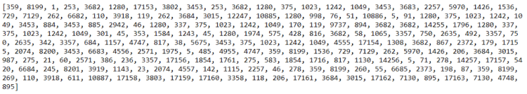
Now that all the texts have been converted into sequence of numbers which is stored in all_encoded_texts array. Here’s how the encoded version of our first news article looks like.

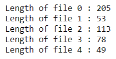
But again, the text preprocessing step hasn’t finished yet! Notice that all files are having different lengths. We can either check it by opening the files manually or using a simple code like this:

for i in range(5):
    print('Length of file', i, ':', len(all_encoded_texts[i]))

In order for machine learning algorithms to work, we need to modify those files such that all of those are having the exact same length. My approach here is to employ pad_sequences() function taken from Keras module. Also, in this project I decided to limit each data sample to 500 words. Zero padding will be added to the beginning of the file which contains less than 500 words.

all_encoded_texts = sequence.pad_sequences(all_encoded_texts, maxlen=500)

Now if we try to print the shape of all_encoded_texts, we are going to obtain the following output:

(3732, 500)

It essentially tells us that we are now having 3732 data samples in which each of those consists of 500 words in length. Finally, that’s all of the text preprocessing! Now that this all_encoded_texts array is going to be our features (X data).

Label preprocessing

We have already got our X data for the training process in the previous stage. Now in this part, we need to define our ground truth — or, also known as label. The idea here is that I wanna create another array which has the exact same length as our X data, yet this one stores the class name of each sample. For the sake of simplicity, we are just going to encode the class name manually, where computer graphics, motorcycles, medical science and politics will be encoded as 0, 1, 2 and 3 respectively.

labels_0 = np.array([0] * len(class_0))
labels_1 = np.array([1] * len(class_1))
labels_2 = np.array([2] * len(class_2))
labels_3 = np.array([3] * len(class_3))

Also, we will concatenate all those separated labels into a single array using np.append() — exactly the same as what we’ve done to concatenate the actual texts.

all_labels = np.append(labels_0, labels_1)
all_labels = np.append(all_labels, labels_2)
all_labels = np.append(all_labels, labels_3)

If we check the shape of this all_labels variable, then we are going to obtain the value of 3732 — which is also exactly the same as the number of X data.

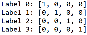
Furthermore, we still need to convert those labels into one-hot representation. This step is done because that’s just what a neural network expect in multi class classification task. For those who are still not familiar with one-hot, it’s essentially looks like this:

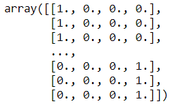
In order to convert our labels to be in such form, we can simply use OneHotEncoder() object. Notice the code below that I use np.newaxis to create a new axis before fitting the one-hot encoder. Well, this is done just because OneHotEncoder() works with that additional axis.

all_labels = all_labels[:, np.newaxis]

one_hot_encoder = OneHotEncoder(sparse=False)
all_labels = one_hot_encoder.fit_transform(all_labels)

Now if you print all_labels, the result is gonna look something like the following figure.

That pretty much it about label preprocessing stage! Keep in mind that all_labels array is going to be our y data. We are going to use both X and y in the next stage — well, certainly 🙂

Model training

There are several things to do in the model training stage. First, we need to split the data into train/test. This is pretty important to find out whether our model is overfitting during the training process. Luckily, we got a train_test_split() function which is taken from Scikit-Learn module. In this case I decided to use 20% of samples in the dataset as the test data while the rest is going to be used for training. Additionally, it’s good to know that when we use this train_test_split() function we no longer need to shuffle the data since the function does it automatically for us.

X_train, X_test, y_train, y_test = train_test_split(all_encoded_texts, all_labels, test_size=0.2, random_state=11)

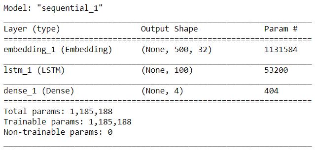
Now, let’s begin to construct the neural network by defining a Sequential() model which then followed by adding 3 layers.

model = Sequential()

model.add(Embedding(input_dim=35362, output_dim=32, input_length=500))
model.add(LSTM(100))
model.add(Dense(4, activation='sigmoid'))

The first layer that we put in the neural network model is an embedding layer. The arguments of that layer are vocabulary size (as the input_dim), vector size (as the output_dim) and input length respectively. In this case, we can take the vocabulary size from the length of tokenizer.word_index, which shows that we got 35362 unique words in our dictionary. The vector size itself is free to choose, here I decided to represent each word in 32 dimensions — well this is essentially the main purpose of using an embedding layer. The last argument I think is pretty straightforward — it’s the number of words of each text sample. Here’s an article if you wanna read more about embedding layer.

The second layer to add consists of 100 LSTM cells. This type of neuron is commonly used to perform classification on sequential data. This is because an LSTM cell does not treat every data point (in this case a data point is a word) as an uncorrelated sample. Instead, input in the previous time steps will also be taken into account to update cell state and the next output value. Well, that’s just an LSTM explanation in a nutshell. If you are interested to understand the underlying math I suggest you to read it from this article.

Lastly, we will connect this LSTM layer with a fully-connected layer which contains 4 neurons where each of those are used to represent a single class name.

Now before the training process begin we need to compile the model like this:

model.compile(loss='categorical_crossentropy', 
              optimizer='adam', 
              metrics=['accuracy'])

In this case, I use categorical cross entropy loss function in which its values is going to be minimized using Adam optimizer. This loss function is chosen because this classification task has more than 2 classes. To the optimizer itself, I choose Adam since in many cases it just works better than any other optimizers. Below is the summary of our model looks like:

Now as the neural network has been compiled, we can start the training process. Notice that I store the learning history in history variable.

history = model.fit(X_train, y_train, epochs=12, batch_size=64, validation_data=(X_test, y_test))

Here is how my training progress goes:

Train on 2985 samples, validate on 747 samples
Epoch 1/12
2985/2985 [==============================] - 75s 25ms/step - loss: 1.3544 - accuracy: 0.3652 - val_loss: 1.2647 - val_accuracy: 0.6466
.
.
.
Epoch 5/12
2985/2985 [==============================] - 48s 16ms/step - loss: 0.4278 - accuracy: 0.9196 - val_loss: 0.4589 - val_accuracy: 0.8768
.
.
.
Epoch 9/12
2985/2985 [==============================] - 49s 16ms/step - loss: 0.1058 - accuracy: 0.9759 - val_loss: 0.1859 - val_accuracy: 0.9438
.
.
.
Epoch 12/12
2985/2985 [==============================] - 49s 16ms/step - loss: 0.0253 - accuracy: 0.9966 - val_loss: 0.1499 - val_accuracy: 0.9625

For the sake of simplicity, I decided to delete several epochs. But don’t worry, you can still see the training process history using the following code (both accuracy and loss value).

plt.figure(figsize=(9,7))
plt.title('Accuracy score')
plt.plot(history.history['accuracy'])
plt.plot(history.history['val_accuracy'])
plt.legend(['accuracy', 'val_accuracy'])
plt.show()

plt.figure(figsize=(9,7))
plt.title('Loss value')
plt.plot(history.history['loss'])
plt.plot(history.history['val_loss'])
plt.legend(['loss', 'val_loss'])
plt.show()

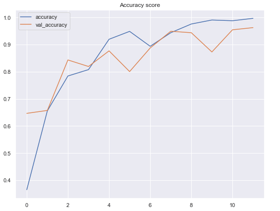
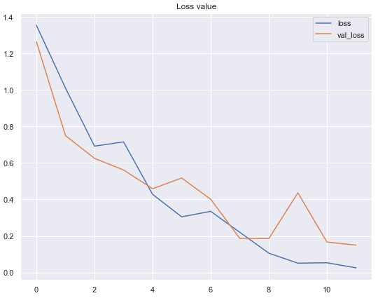
According to the 2 graphs above, we can see that the performance of our neural network classifier is pretty good. The model achieves 99.7% of accuracy on training data and 96.3% on test data. In fact, I’ve tried to increase the number of epochs to see whether the performance can still be improved. However, somehow the accuracy on both data are just fluctuating randomly at around 90% to 97%. So then I decided to restart the training and stop at epoch 12.

Model evaluation

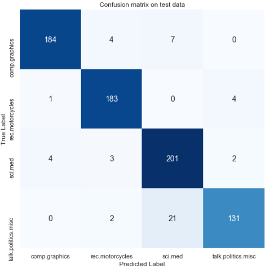
Now we are going to get deeper into the model evaluation. To me, understanding the accuracy and loss value graphs is not enough. I do prefer to construct a confusion matrix and see which class causes the neural net classifier getting confused.

To do that, let’s begin with predicting our X_test data. The first line of the code below returns something like a probability value — yet it’s important to keep in mind that it’s actually not a probability since our output layer is using sigmoid activation function, not a softmax. But still, the idea is to take the highest value as the predicted class, which is done in the second line of the code below.

predictions = model.predict(X_test)
predictions = one_hot_encoder.inverse_transform(predictions)

The next thing to do is to convert our labels back from one-hot format. My approach here is to use np.argmax() function and store the non-one-hot format in y_test_evaluate array.

y_test_evaluate = np.argmax(y_test, axis=1)

Now as the values of predictions and ground truth are already comparable, so we can directly use confusion_matrix() function taken from Sklearn module. Remember that the arguments of this confusion matrix are the actual value and the predicted value respectively.

cm = confusion_matrix(y_test_evaluate, predictions)

Finally, we can just draw the confusion matrix by passing cm variable as the argument of heatmap() function. We can see the result below that strangely most of the errors here are in the politics texts. It shows that there are 21 politics-related news which are misclassified as medical science text.

plt.figure(figsize=(8,8))
plt.title('Confusion matrix on test data')
sns.heatmap(cm, annot=True, fmt='d', xticklabels=labels, yticklabels=labels, 
            cmap=plt.cm.Blues, cbar=False, annot_kws={'size':14})
plt.xlabel('Predicted Label')
plt.ylabel('True Label')
plt.show()

Now what if we got a new string and we want to find out which class should this text belong to? There are several steps required to do so. First lemme create a string like this:

string = 'I just purchased a new motorcycle, I feel like it is a lot better than cars'

We know that the text is actually pretty clean. However, notice that there are still several stop words in which may not be important in the text above. Hence, we will pass this text into our clean() function that we defined in the earlier part of this writing.

cleaned_string = clean(string)

The next thing to do is to encode those texts into numbers and store the result in encoded_string variable.

encoded_string = tokenizer.texts_to_sequences([cleaned_string])

Now, remember that the encoded text above only consists of 8 words. We can not directly feed this into our neural network since it takes exactly 500 words in order to work. Thus, we are going to add zeros in front of this text such that there will be 500 encoded values in the string. We can simply do this using pad_sequences() function and set the maxlen argument to 500.

encoded_string = sequence.pad_sequences(encoded_string, maxlen=500)

I don’t wanna display the screenshot of the encoded_string here because it takes plenty of space. Just print that out yourself and you’ll see how it looks like.

As the string has been at the exact same size as our trained model input, we can now start doing the prediction and store the probability-like value to the string_predict variable. Lastly we can take the argmax of string_predict value to find out the prediction made by our neural network model on our own data.

string_predict = model.predict(encoded_string)
np.argmax(string_predict)

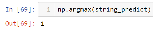
We can see here that the prediction is right! The string that we are using to test this sample is highly related to motorcycle, and our neural net predicts it correctly.

That’s pretty much about today’s article. Let me know your opinion regarding to this project in the comment section below. Thanks for reading and see you!

Note: here’s the code used for this project:

References

Illustrated Guide to LSTM’s and GRU’s: A step by step explanation by Michael Phi https://towardsdatascience.com/illustrated-guide-to-lstms-and-gru-s-a-step-by-step-explanation-44e9eb85bf21

What is an Embedding Layer? by Georgios Drakos https://gdcoder.com/what-is-an-embedding-layer/#:~:text=The%20first%20argument%20(8)%20is,that%20we%20used%20for%20padding.

Don’t forget to give us your ? !

---

News Topic Classification using LSTM was originally published in Becoming Human: Artificial Intelligence Magazine on Medium, where people are continuing the conversation by highlighting and responding to this story.

Via https://becominghuman.ai/news-topic-classification-using-lstm-a1e8a38781fe?source=rss—-5e5bef33608a—4

A Systematic Assessment of National Artificial Intelligence Policies: Perspectives from the Nordics and Beyond

By analysing 25 national AI policy documents, we identified differences in national prioritisation of AI related topics. For example, Sweden’s strategy has a strong focus on research, Japan on collaboration, and Serbia and France on ethical frameworks. Geographical clusters, such as the Northern Countries or the Anglosphere, are closely aligned in terms of ethical prioritisation, highlighting opportunities for future collaboration and geographical diversification of AI applications.

This entry summarises our NordiCHI 2020 paper “A Systematic Assessment of National Artificial Intelligence Policies: Perspectives from the Nordics and Beyond” by Niels van Berkel, Eleftherios Papachristos, Anastasia Giachanou, Simo Hosio, and Mikael B. Skov.

The increasing impact of Artificial Intelligence (AI) on the everyday life of individuals and organisations has led many governments to take an increasingly active role in the assessment and support of new AI applications. Governments have stressed that AI applications should reflect national values, as for example seen in The White House’s push for “AI with American values”. In order to better understand the differences in how national governments position themselves on this emerging agenda, we set out to analyse national strategy and policy documents.

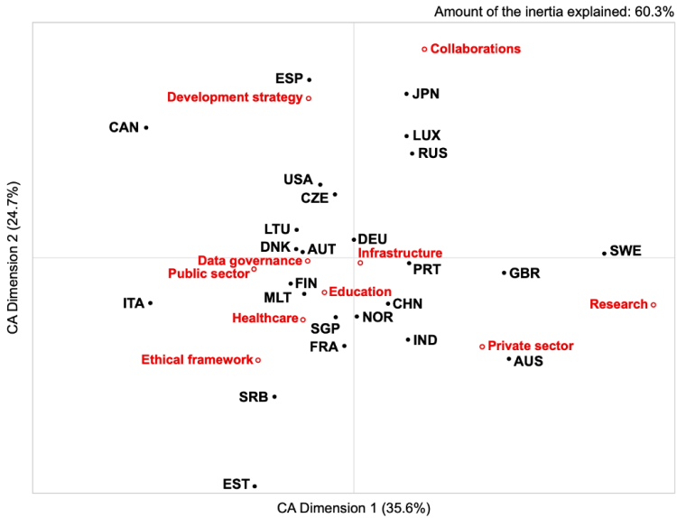
Through a systematic search, we identified 25 national policy documents. We applied a text analysis technique known as Latent Dirichlet Allocation to these documents to identify the topics that were discussed, identifying ten distinct topics;

1. Development strategy
2. Infrastructure
3. Private sector
4. Public sector
5. Data governance
6. Ethical framework
7. Education
8. Healthcare
9. Collaboration
10. Research.

We subsequently assessed the relative frequency with which these topics were discussed within each nation’s AI policy. Figure 2 highlights how the national policies are aligned to each topic, with closer proximity to a topic indicating that the topic was covered more extensively by the country. Countries at the extreme are quite unique in the focus they gave to specific topics. For example, Japan’s policy focuses more strongly on collaborations as compared to the other countries. Similarly, Spain focused more on development strategies, Serbia and France on ethical frameworks, Australia on the Private sector, and Sweden on Research than the rest of the countries.

Trending AI Articles:

1. Microsoft Azure Machine Learning x Udacity — Lesson 4 Notes

2. Fundamentals of AI, ML and Deep Learning for Product Managers

3. Roadmap to Data Science

4. Work on Artificial Intelligence Projects

Strategy & Ethics

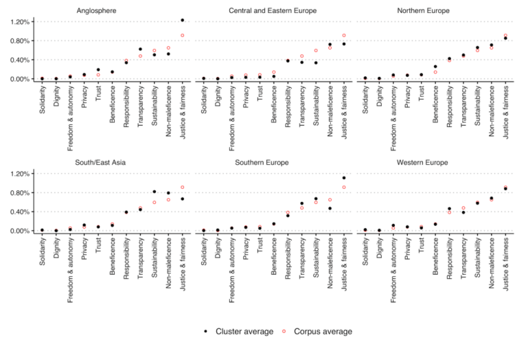
Whether or not AI behaves ethically and in line with our (moral) expectations is an often discussed topic both within popular media and academia. For a set of eleven ethical principles (e.g., transparency, sustainability), we assess the frequency with which they are discussed in each policy document. By grouping the documents in six geographical clusters, we aim to assess differences in the perspective of cultural or geographical clusters on the ethical concerns of AI. Figure 3 presents, for each of the six clusters, the average frequency with which the ethical principles are discussed. Countries within the Anglosphere cluster, for example, focus more heavily on ‘Justice & fairness’ than the entire collection of policy documents as a whole (called ‘corpus’). The South/East Asia cluster, on the other hand, highlights a stronger focus on ‘Sustainability’ and ‘Non-maleficence’.

Reading the documents manually also uncovers some of the differences between countries. Ethic documents from the cluster of Northern European countries often refer to pre-existing cultural conditions as a base for expanding their AI efforts;

“Finland is known for its high level of citizen trust […] It is a privilege to step into the age of artificial intelligence from such an exceptional setting. At the same time, it practically obliges us to an active approach, understanding of the prerequisites of trust in the age of artificial intelligence […].”
 — Final report of Finland’s Artificial Intelligence Programme

“Norwegian society is characterised by trust and respect for fundamental values such as human rights and privacy. This is something we perhaps take for granted in Norway, but leading the way in developing human-friendly and trustworthy artificial intelligence may prove a key advantage in today’s global competition.”
 — Norway’s National Strategy for Artificial Intelligence

Our results highlight key differences between the analysed country’s (ethical) priorities regarding AI development. Using automated text analysis methods, we identify geographical clusters which align with existing cultural groupings. This highlights the opportunity for countries to cooperate on their AI research and development efforts with culturally aligned partners. Understanding the differences in perspectives towards AI technology between countries is a first step towards ensuring that AI applications align with the values of end-users cross-culturally.

“Europe and Denmark should not copy the US or China. Both countries are investing heavily in artificial intelligence, but with little regard for responsibility, ethical principles and privacy”.
 — Denmark’s National Strategy for Artificial Intelligence

If you found this story interesting, please read the paper or contact one of the authors! We also recommend Jobin et al.’s paper “The global landscape of AI ethics guidelines”, which inspired our work.

Paper citation: N. van Berkel, E. Papachristos, A. Giachanou, S. Hosio, M. B. Skov, “A Systematic Assessment of National Artificial Intelligence Policies: Perspectives from the Nordics and Beyond”, Proceedings of the 11th Nordic Conference on Human-Computer Interaction (NordiCHI’20), 2020. doi: 10.1145/3419249.3420106.

Don’t forget to give us your ? !

---

A Systematic Assessment of National Artificial Intelligence Policies: Perspectives from the… was originally published in Becoming Human: Artificial Intelligence Magazine on Medium, where people are continuing the conversation by highlighting and responding to this story.

Via https://becominghuman.ai/a-systematic-assessment-of-national-artificial-intelligence-policies-6db97306be70?source=rss—-5e5bef33608a—4